1. Introduction
Among many others, surface acoustic wave (SAW) sensors are widely used in various fields of application [
1,
2]. SAW sensors for measuring temperature [
3,
4], pressure [
5,
6], electric fields [
7], magnetic fields [
8,
9], humidity [
10], and vibration [
11], or for the detection of gases [
12] and biorelevant molecules [
13,
14], respectively, have been reported.
In this paper, two-port sensors are considered that consist of one input and one output interdigital transducer (IDT) structured on the piezoelectric substrate to convert efficiently between electrical and mechanic waves [
15]. Two SAW device structures are most widely used. A delay line essentially consists of two IDTs placed some distance apart, whereas a resonator has additional reflector gratings to confine the wave energy inside a resonant cavity ([
16], p. 141). In most cases, the SAW device is coated with a certain material that interacts with the physical quantity to be measured and, in turn, leads to an alteration of the wave propagating along the substrate’s surface. Thus, the transceived signals of such coated sensors are generally modulated in phase and in amplitude.
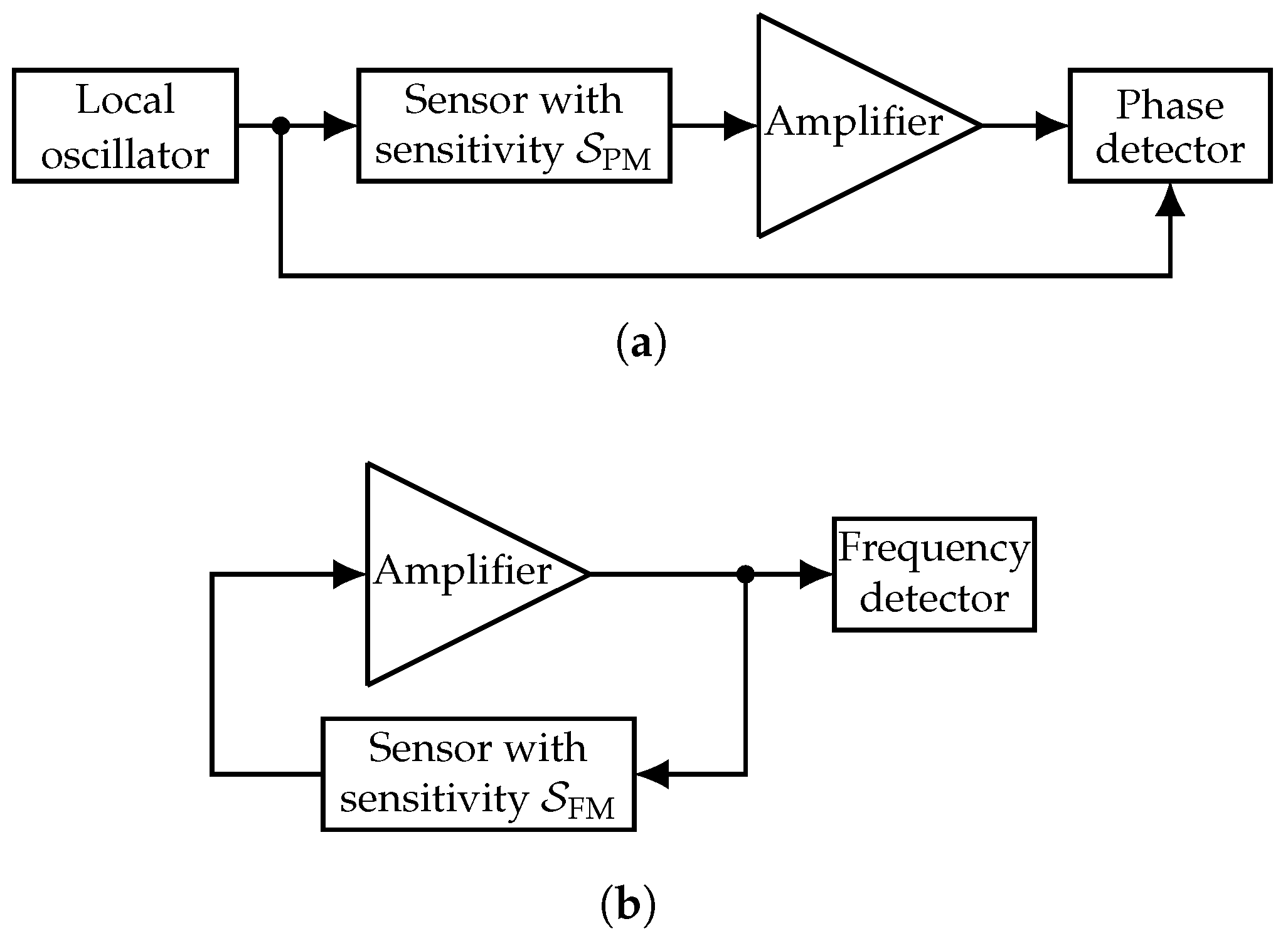
For the readout of SAW sensors, two structures are most common. A straightforward approach is to compare the sensor’s output signal with a local oscillator (LO) signal fed into the sensor in an open-loop configuration [
17]. Such systems not only allow for the detection of both amplitude and phase changes like with a vector network analyzer (VNA), but are also suited for the characterization of the frequency response of the sensor. However, especially due to the needed LO, these systems are often complex [
18,
19]. In the most common readout structure, the SAW sensor is inserted into the feedback loop of an amplifier, thus forming a closed-loop system in which the oscillating signal is frequency modulated when the phase response of the sensor changes [
20,
21,
22]. Such systems appear to be simple [
23,
24], but mostly also require a reference oscillator for the frequency detection. In addition, a self-oscillating sensor system is, without introducing additional expense, usually only suitable for the detection of changes in the sensor’s phase response because variations in the oscillator signal’s amplitude are strongly suppressed by the saturation of the internal amplifier.
In general, depending on the application of a sensor system, properties like, e.g., bandwidth, dynamic range, linearity, and immunity against environmental influences are required. However, for high-end sensor systems, the limit of detection (LOD) is often the most important figure of merit. In this paper, open-loop and closed-loop sensor readout systems are investigated and compared in terms of the achievable LOD.
This paper is organized as follows:
Section 2 introduces open-loop and closed-loop readout systems for both resonant and delay line sensors. In
Section 3, expressions for describing the phase noise behavior of both readout systems and for both types of sensors are derived. Based on these results, the LOD for the various cases are calculated in
Section 4 where the equivalence of the LOD between open-loop and closed-loop systems is shown. This article finishes with an additional consideration of the time domain uncertainty in
Section 5 and a summary of the findings in
Section 6.
3. Phase Noise
Assuming an arbitrary signal
that describes the physical quantity to be measured in units of
, the phase-modulated signal in an open-loop system can be expressed as:
where the carrier signal with the frequency
is impaired by random phase fluctuations
in units of
due to phase noise introduced by the readout electronics and by the sensor itself. The frequency-modulated signal in a closed-loop system is also impaired by random phase fluctuations
in units of
:
which can, alternatively, also be described by random frequency fluctuations
in units of
:
With the instantaneous frequency being the time derivative of the phase, the relation between random phase fluctuations and random frequency fluctuations in the time domain [
29] is given by:
In general, arbitrary random phase fluctuations
are best described by the one-sided power spectral density
of the random phase fluctuations. An equivalent and widely-used representation is
, which is defined as
[
30]. However,
is used throughout this paper because it is given in SI units of
and thus makes further conversions more straightforward. A model that has been found useful in describing the frequency dependence of a power spectral density of random phase fluctuations is the power law:
with usually
.
and
refer to white phase noise and
flicker phase noise, respectively, which are the main processes in two-port components ([
28], p. 23, [
31]). As will be shown further below, in closed-loop systems, white phase noise results in white frequency noise (
), and flicker phase noise results in flicker frequency noise (
). Higher order effects like random walk of frequency (
) are related to environmental changes like, e.g., temperature drifts, humidity, and vibrations [
29].
The term
quantifies the constant, i.e., white, phase noise floor where
F is the noise figure and
is the thermal energy. This type of noise is additive, which means that
F does not change when a carrier signal with power
is injected into the according component. When, e.g., a sensor and an amplifier are cascaded, the overall phase noise at the output depends on the individual gains and can be calculated by an adaption of the well-known Friis formula [
28,
31]. Flicker phase noise is always present, described by the term
. It is a form of parametric noise because the carrier is modulated by a near-DC flicker process. Experiments show that
is almost independent of carrier power
; thus, the Friis formula does not apply for cascaded two-port components showing flicker phase noise. Instead, the flicker phase noise, i.e., the coefficients
of the individual components, just adds up [
31].
Phase modulation is difficult to model. Therefore, we transform the radio frequency (RF) schemes into their phase-space equivalent, which is a linear representation where the signal is the phase of the original RF circuit. This transformation is shown for the open-loop system in
Figure 3 and for the closed-loop system in
Figure 4, respectively, and extensively discussed later. It is assumed that the gain
A of the amplifiers is constant in the frequency range around the sensor’s center frequency. Thus, in the phase-space representation, an amplifier simply repeats the input phase to its output and has a gain exactly equal to one [
32]. For the frequency-dependent transfer function of the sensor in the Laplace domain
with the complex angular frequency
, the equivalent phase-space representation
is calculated with the phase-step method ([
28], p. 103 ff., [
33], Section 4). This method is based on the well-known property of linear time-invariant (LTI) systems for which the impulse response is the derivative of the step response and the system’s transfer function is the Laplace transform of the impulse response. Thus, the phase-space representation of the sensor’s transfer function:
is the Laplace transform of the derivative of the phase step response
, which follows as part of the output signal
when, in turn, a phase step
with
as part of the input signal
is fed into the sensor. With
, linearization is obtained that is physically correct for phase noise being usually very small. The term
is the unit-step function also referred to as the Heaviside function.
For a resonant sensor with the angular natural frequency
, which can be described by the general transfer function:
the phase-space representative is given by:
The according magnitude-squared transfer function yields:
The magnitude frequency response of a SAW delay line device is occasionally described using a sinc function
, where
is a correction factor ([
34], p. 80). Such a function properly can take into account the steepness of the bandpass characteristic and transmission zeros. However, because SAW sensors are always operated in their passband, calculations in this paper are simplified by choosing the transfer function of a bandpass filter to describe the sensor. With the angular center frequency
, the SAW delay line sensor’s frequency response then yields:
which results in a phase-space representative given by:
The according magnitude-squared transfer function yields:
3.1. Phase Noise in the Open-Loop Readout System
Figure 3a depicts the open-loop readout system in the RF domain together with the random phase fluctuations of the input voltage, i.e., the LO,
, the sensor
, and the amplifier
. The related power spectral densities are denoted by
,
, and
. As described above, the phase-space representation of the system (
Figure 3b) is more suited to calculate the overall phase noise at the output of the open-loop system
. Due to linearity, the Laplace transforms of the phase noise of the sensor
and the amplifier
can be arranged in front of the phase-equivalent sensor
. Thus, the phase noise transfer function for both the sensor and the amplifier to the output of the system:
is equal to
where
. For the phase noise of the LO
, the phase noise transfer function to the output of the open-loop system is given by:
Thus, the overall power spectral density of the random phase fluctuations at the output of the open-loop sensor system as a function of both the phase noise of the individual components and the frequency response of the sensor yields:
The magnitude-squared transfer functions
and
in Equation (
21) depend on the type of sensor and are derived in the following.
3.1.1. Resonator
For a resonant sensor, the power spectral densities of the random phase fluctuations of the sensor and the amplifier are simply weighted by
(Equations (
15) and (
19)). According to Equation (
20), the transfer of the phase noise of the LO to the output of the system is given by:
Both phase noise transfer functions as a function of the frequency and for various quality factors are visualized in
Figure 5a. As expected, the phase noise of the sensor and the amplifier will be transformed unaltered to the open-loop system’s output for frequencies inside the sensor’s passband (green curves). The −3dB cutoff frequency
is called the Leeson frequency ([
28], p. 74), which is equal to half of the resonator’s bandwidth
. The phase noise of the oscillator is largely suppressed for low frequencies and low quality factors. However, both for increasing frequency and increasing quality factor, the suppression decreases (blue curves). The reason is that the correlation of LO phase noise in both branches of the open-loop system decreases for higher frequencies and for longer relaxation time of the resonator.
3.1.2. Delay Line
For a delay line sensor in an open-loop system, the power spectral densities of the random phase fluctuations of the sensor and the amplifier are weighted by
(Equation (
18)). According to Equation (
20), the transfer of the phase noise of the LO to the output of the system is given by:
The exact result in Equation (
23) takes into account the finite bandwidth of the sensor. For frequencies inside the sensor’s passband (
), the expression distinctly simplifies and gives the same result calculated following another approach and verified by measurements in previous investigations [
25]. All three phase noise transfer functions are depicted in
Figure 5b. As for the previously-discussed resonant sensor, the phase noise of the sensor and the amplifier will be transformed unaltered to the open-loop system’s output for frequencies inside the sensor’s passband (green curves), i.e., the −3dB cutoff frequency
. The phase noise of the oscillator (dark blue curved), again, is largely suppressed for low frequencies, which, inside the sensor’s passband, is well described by the approximation in Equation (
24) (dashed light blue curves). Because of the decreasing correlation of the LO phase noise in both branches of the open-loop system for higher delay times, the suppression decreases with
.
3.2. Phase Noise in the Closed-Loop Readout System
Figure 4a depicts the closed-loop readout system, i.e., the oscillator, in the RF domain together with the random phase fluctuations of the sensor
and the amplifier
. The related power spectral densities are denoted by
and
. As described above, the phase-space representation of the system (
Figure 4b) is more suited to calculate the overall phase noise at the output of the closed-loop system
. Due to linearity, the Laplace transforms of the phase noise of the sensor
and the amplifier
can be arranged at any point inside the loop. Elementary feedback theory known from, e.g., classical control theory or the analysis of operational amplifier circuits yields the phase noise transfer function of the closed-loop system:
Thus, the overall power spectral density of the random phase fluctuations at the output of the oscillator as a function of both the phase noise of the sensor and the amplifier and the characteristic of the sensor yields:
According to the relation between random phase fluctuations and random frequency fluctuations in the time domain in Equation (
10), the power spectral density of the random frequency fluctuations at the output of the oscillator in units of
is given by:
In Equation (
26) and also for Equation (
27), the magnitude-squared phase noise transfer function
depends on the type of sensor and is derived in the following.
3.2.1. Resonator
According to Equation (
25), for a resonant sensor with the phase-space equivalent transfer function
from Equation (
14), the phase noise transfer function of the closed-loop system yields:
Thus, the magnitude-squared phase noise transfer function that transforms the power spectral densities of the random phase fluctuations of the resonant sensor and the amplifier into oscillator phase noise (Equation (
26)) results in:
This equation is equal to the well-known Leeson formula [
35], which simplifies to:
for slow phase fluctuations below the Leeson frequency. As can be seen in
Figure 5a, the phase noise of the sensor and the amplifier is strongly raised in the closed-loop and even increases with the quality factor
Q. This phenomenon is known as the Leeson effect.
3.2.2. Delay Line
According to Equation (
25), for a delay line sensor with the phase-space equivalent transfer function
, from Equation (
17), the phase noise transfer function of the closed-loop system yields:
Thus, the magnitude-squared phase noise transfer function that transforms the power spectral densities of the random phase fluctuations of the delay line sensor and the amplifier into oscillator phase noise (Equation (
26)) results in:
As for resonant sensors, in closed-loop systems, the phase noise of the sensor and the amplifier is strongly raised and increases with the delay time
(
Figure 5b).
5. Time Domain Uncertainty
The sensor system’s output is most often exploited as a continuous stream of values:
each averaged over a suitable time
with
(please do not confuse
with the delay time of a delay line sensor
or the relaxation time of a resonant sensor
). It is therefore appropriate to describe the sensor system’s noise in terms of a two-sample variance, also called Allan variance (AVAR) [
36,
37], which is defined as:
where
and
are two values of
averaged on contiguous time slots of duration
and
denotes the mathematical expectation operator. Using a weighted average in Equation (
45) results in other types of variances, like the modified Allan variance [
38,
39], the parabolic variance [
40,
41], etc., which are less common for sensors. Traditionally,
is the fractional frequency fluctuation
. However, the AVAR is a general tool, and
can be replaced with any quantity, either absolute or fractional. In all experiments, the expectation
is replaced with the average on a suitable number of realizations. The Allan variance can be seen as an extension of the classical variance, where the low-pass effect resulting from the difference
provides the additional property that the AVAR converges for flicker and random walk processes, and even for a linear drift. These processes are of great interest for oscillators and sensor systems. Interestingly, random walk and drift in electronics are sometimes misunderstood, and both described with a single parameter called aging (see for example [
42]). The quantity
is the statistical uncertainty, also referred to as Allan deviation (ADEV), which depends on the measurement time
(
Figure 7) and can be calculated from the power spectral density
of random fluctuations of
y (
Table 2).
The uncertainty decreases proportionally with for white noise processes and attains its minimum in the flicker region where the uncertainty is independent of . This identifies as the optimum measurement time, to the extent that the lowest uncertainty is achieved in the shortest measurement time. Beyond , the uncertainty degrades.
At the output of the sensor system, the quantity of interest is represented by a phase in the case of the open-loop system and represented by a frequency in the case of the closed-loop system, i.e., the oscillator. Consequently, the optimum measurement time
is given by the intercept point between white phase noise (
) and flicker phase noise (
) for the open-loop system and by the intercept point between white frequency noise (
) and flicker frequency noise (
) for the closed-loop system, respectively. Following the expressions for the power spectral densities of random phase fluctuations
(Equation (
21)) and random frequency fluctuations
(Equation (
27)), the coefficients
and
result in expressions as listed in
Table 3 when considering only the phase noise of the sensor as
. Thus, the optimum measurement time:
turns out to be the same for open-loop and closed-loop systems, as well as for both types of sensors. Our conclusion, that the two measurement methods are equivalent, relates to the sensor systems only, assuming that these are ideal. However, the shown derivations can be easily extended for
and
, at least numerically. It turns out that the background noise of a phase detector (used for the differential phase measurement in the open-loop system) is lower than the background of a frequency detector, i.e., a frequency counter. The reason is that the phase meter is a dedicated device, specialized for the phase detection in a narrow range around a given frequency. Overall, this kind of measurement relies on the principle of a lock-in amplifier, whose bandwidth is determined by a low-pass filter. By contrast, a frequency counter is a general-purpose device suitable for a wide range of input frequencies. Consequently, the statistical uncertainty is affected by the wide noise bandwidth.


