In this section, a novel approach based on game theory is proposed to address the problem of barrier coverage for dynamic monitoring systems. This method proved to be a potential game and a heuristic solution to the DBC problem. It can converge into Nash equilibrium using a new distributed learning algorithm.
4.1. Rational Game Theory
In the game of DBP formation, each sensor, as a participant, selfishly wants to maximize its own benefits based on local information gathered from the network and actions taken by other participants. The effective benefits of each participant depend not only on its own behavior, but also on the actions taken by other participants.
When each participant chooses its own optimal action strategy, no one will actively deviate from its current strategy choice when other participants’ strategy remains unchanged. At this time, the strategy combination of each player is called Nash equilibrium. In addition, by designing an appropriate utility function, each sensor gets the best benefit, and the DBC problem can also obtain the global optimal solution.
Definition 6. Nash equilibrium [38]. Suppose a strategy game Γ (V, S, u) has a combinatorial strategy(,)S forviV, iN and if there is a siS forviV satisfies Equation (12), the combinatorial strategy(,) is a Nash equilibrium of the game Γ,where i represents participant i, and −i represents the remaining N-1 participants of i. A game may have more than one equilibrium, or it may not exist at all. Some types of games have at least one Nash equilibrium. In order to guarantee the existence of Nash equilibrium, a special kind of strategic game-potential game is proposed in [
39], and it is proved that there exists at least one Nash equilibrium.
Definition 7. Ordinal Potential Game (OPG) and Ordinal Potential Function (OPF) [39]. A strategy game Γ (V, S, u) is an OPG if there is a function O (S) that satisfies Equation (13). And the function O (S) is an OPF, Theorem 3 [39]. If the strategy game Γ (V, S, u) is an OPG and O (S) is its OPF, the combinatorial strategy(,) that maximizes O (S) is a Nash equilibrium of the game Γ.
Therefore, if the ordinal potential function of the strategy game is determined, the maximization of the ordinal potential function can be obtained by the combination strategy to obtain the Nash equilibrium of the strategy game.
4.2. Dynamic Barrier Coverage Game Model (DBCGM)
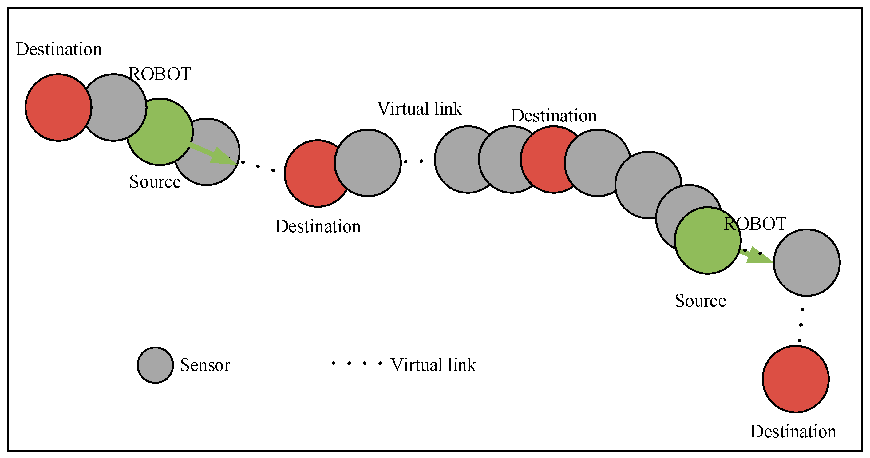
The dynamic barrier coverage game model (DBCGM) based on ordinal potential game is established in this section. In this model, each sensor chooses actions based on its own interests to form DBP. The action (strategy) of each player (sensor) is defined by a vector si as follows: si = κvi Si. A DBP can be regarded as a set of actions Si = (s1, s2, …, sn) S that all players participate in and act on their own interests. It can be expressed as Si = (si, s−i), where s−i = (s1, . . ., si−1, si+1, . . ., sn) refers to all actions taken by all nodes but vi.
Assume that when node
vi takes (deployment/non-deployment) action, the number of deployment actions performed by itself and other nodes within its communication range is
ni (
Si) and
nj (
Si), respectively. Now, the definition of
ni (
Si) and
nj (
Si) for each fixed sensor node in a DBP is as follows,
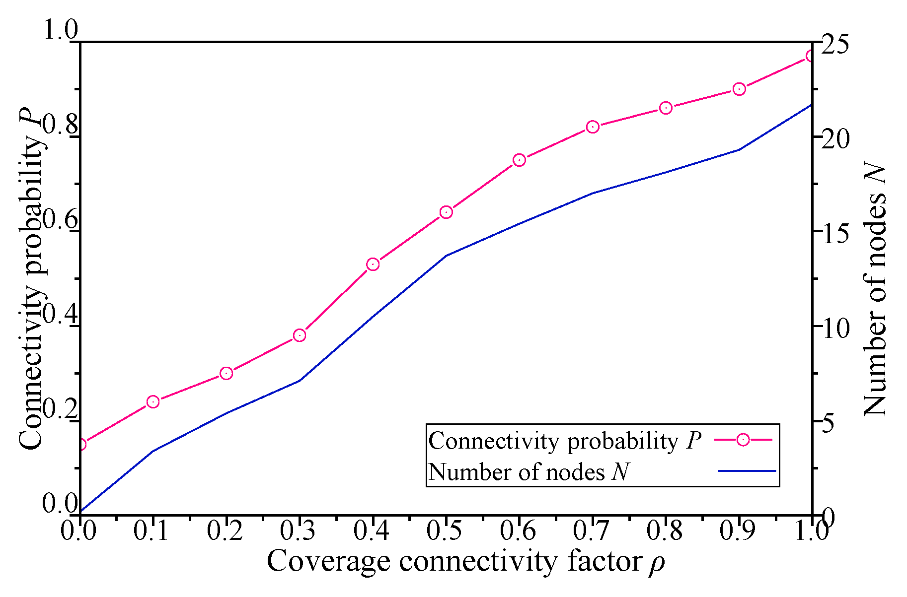
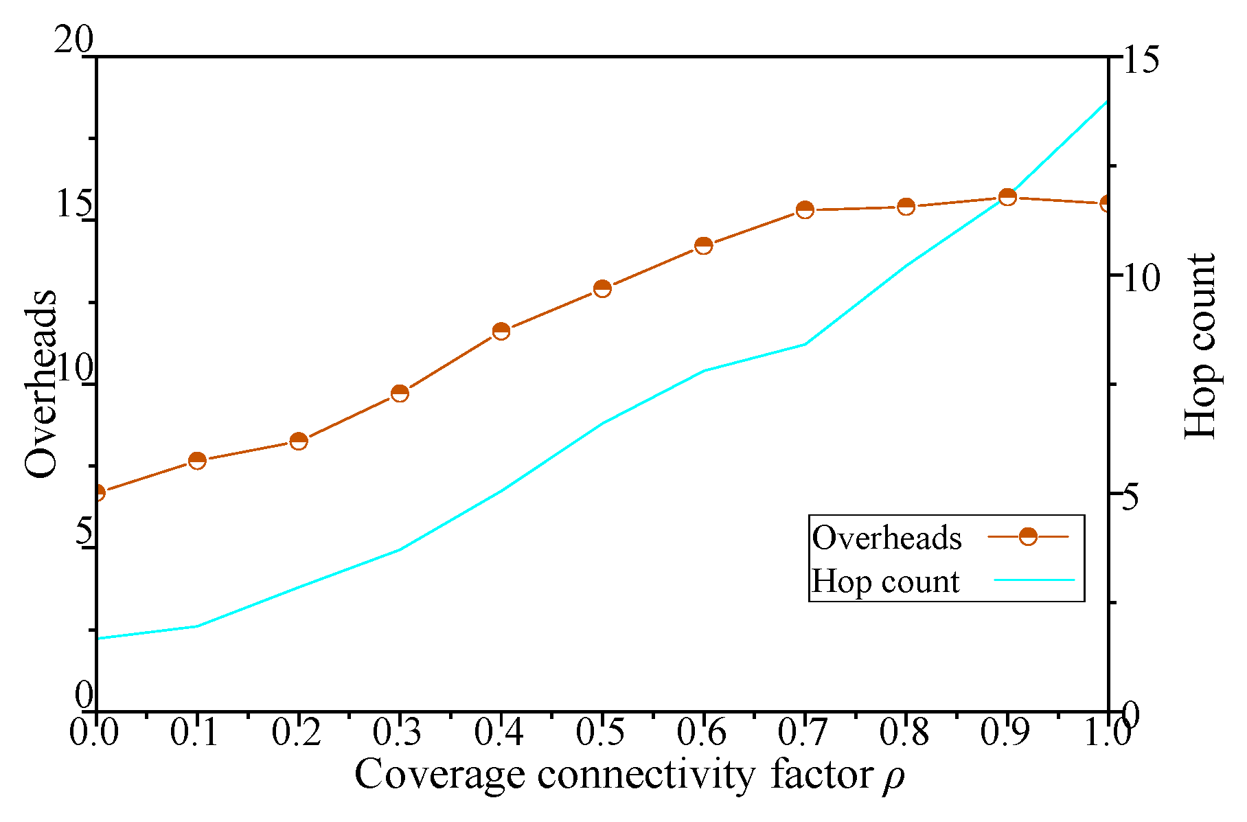
Definition 8. Coverage Connectivity Factor (CCF). The CCF for each DBP is ρ(0,1], which can be preset by different application scenarios. ρ represents the expected goal of connectivity probability for each DBP.
The connectivity probability of DBP under different combination strategies satisfies Equation (16). If
P (
si,
s−i) = 1, the network is connected, that is, node i can communicate with all other nodes through a two-way link, else if
P (
si,
s−i)
(0,1] network shows dynamic intermittent connectivity. Obviously,
P (
si,
s−i) is a monotone nondecreasing function, that is, for any node
vi, as it is deployed or removed (
si1 = 1 >
si2 = 0) in DBP, there is
P (
si1,
s−i) ≥
P (
si2,
s−i),
When nodes transmit messages, the weight average of residual energy for sensors in DBP is given by Equation (17). Where
Ed (
vi) is the residual energy of sensor
vi V, and
Eo (
vi) is the initial energy of sensor
vi V,
The most important step of solving the DBC problem is to determine the utility function of each node
vi V,
i N. The utility function represents the trade-off between the benefits and the cost of each node deploying and connecting to the network. For each DBP, the utility function for the
ith node is defined as,
where
α (0,1] represents the weighting parameter pertinent to the cost and profit. As mentioned above
P (
si,
s−i)
(0,1] is connectivity probability of DBP,
P (
si,
s−i) is positively correlated with the utility function. The greater the value of
P (
si,
s−i), the better the connectivity probability of DBP, and the higher the revenue of static nodes. In the utility function, the product term of
α represents the gain of sensor
vi V under different combination strategy
Si = (
si,
s−i). Under different application premises, by adjusting the size of CCF
ρ, the sensor income value is changed, so that the performance of each node is closely related to the application target.
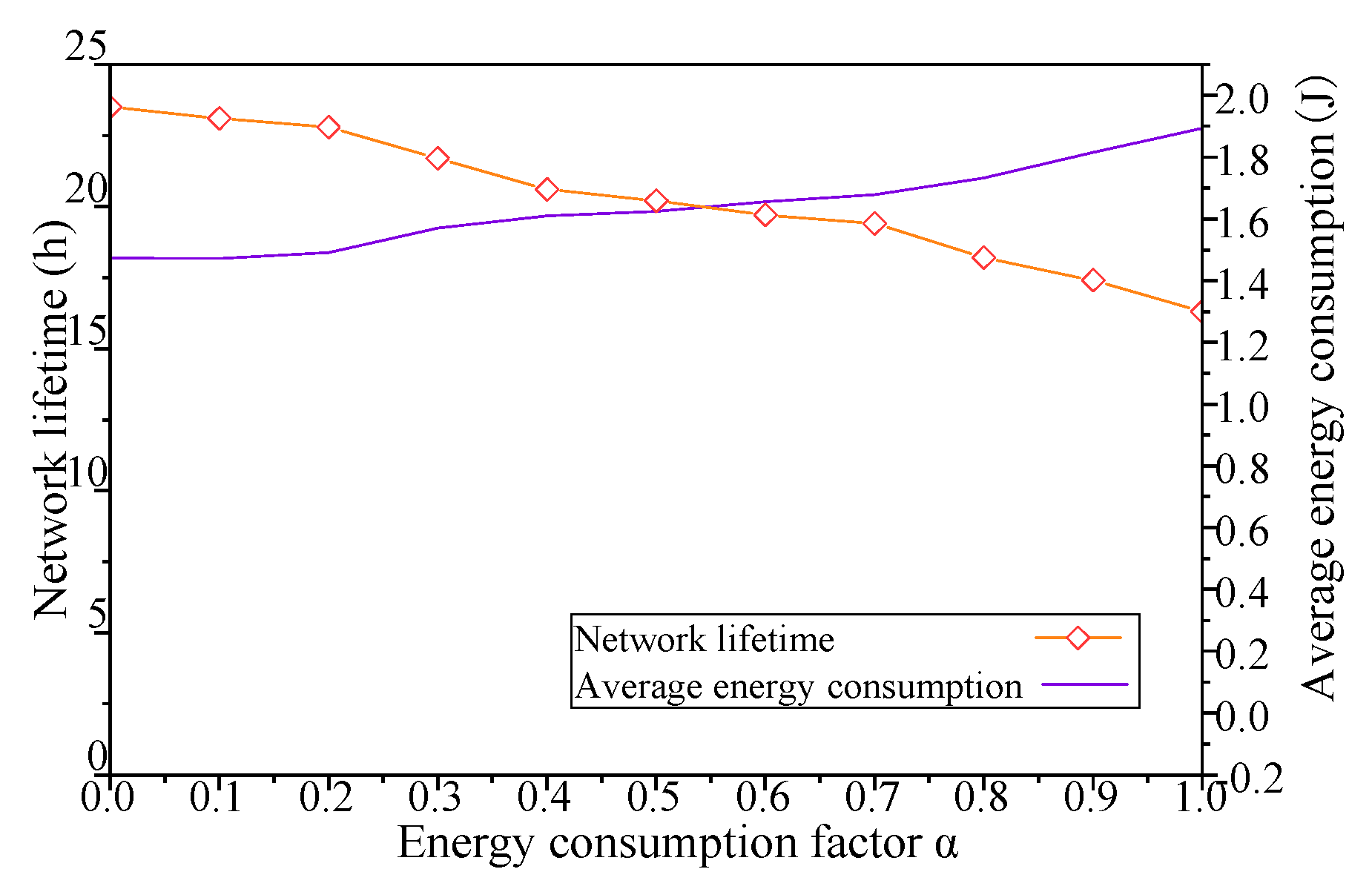
The remaining part of Equation (18) describes the energy consumption of the sensor under the combined strategy Si. E (vi, −i) in the utility function indicates that a node tends to take the node with more residual energy as its neighbor to increase the value of the utility function in order to improve the average residual energy of its neighbor nodes. Energy consumption equalization is very important for optimizing the network topology of maximizing network lifetime. If the energy consumption of the nodes in the network is very uneven, some nodes will run out of energy quickly, which will lead to early termination of the entire network lifetime. The selection strategy based on this utility function helps to balance energy consumption between nodes. In addition, the setting of parameter α can further adjust the proportion of energy consumption to node income. Usually, we use α = 0.5, that is, the way of balancing income and cost to evaluate the node combination strategy.
Theorem 3. The game model of DBC problem is an ordinal potential game. Its ordinal potential function is defined as, Proof of Theorem 3. According to the utility function defined in Equation (19), it is possible to assume that
Si1 and
Si2 are two different strategic actions (
si1 = 1 >
si2 = 0 or
si1 = 0 <
si2 = 1) of node
i, and the difference between the returns of node i when it’s selecting
Si1 and
Si2 respectively is as follows,
Similarly, when node
vi V,
i N selects
Si1 and
Si2 separately, the difference between its ordinal potential functions
Oi is as follows,
Therefore, the following Equation (22) can be obtained,
Since
P (
si,
s−i) is a nondecreasing function, the following Equation (23) is obtained,
In summary, when the initial condition is the same (si1 = 1 > si2 = 0 or si1 = 0 < si2 = 1), sgn (△ui) = sgn (△Oi), i.e., DBCGM, the game model of DBC problem is an ordinal potential game. Its ordinal potential function is Oi.
Inference 1. There must be Nash equilibrium in the Dynamic Barrier Coverage Game Model (DBCGM).
Proof of Inference 1. According to Theorem 3, the function Oi shown in Equation (19) is exactly the ordinal potential function of DBCGM. As can be seen from Theorem 2, the combined strategy of maximizing its ordinal potential function is the Nash equilibrium solution of the model. And any node vi can choose whether to participate in the formation of DBP or not, i.e., the optional strategy si of player vi is limited, so there must be a combination of strategies Si = (si, s−i) that maximizes Oi. This combination of strategies is the solution of the DBCGM.
4.3. Distributed Learning Algorithm
On the one hand, the utility of each player (sensor) is based on the actions taken by itself and other players (especially their neighbors) and their energy performance. On the other hand, since the initial state of network connectivity is uncertain, we assume that each sensor only knows the state of other nodes in its communication range. Therefore, due to the above information constraints, the nodes are unable to calculate the global payoff of a DBP accurately, which associated with alternative actions of each sensor. In addition, on the entire DBP link, only the latest actions that can be contacted locally are available for utility value calculations. Therefore, developing a learning algorithm based on distributed payment is a good option for DBCGM.
In order to solve DBCGM in a distributed way, according to the detailed description of the execution steps of the distributed algorithm, the distributed coverage game algorithm (DCGA) which controls node deployment needs to satisfy the following assumptions:
- (1)
All nodes in the network have unique IDs, which increase from one end of a DBP to the other according to the distribution of DBPs.
- (2)
The connectivity of the whole DBP can be judged in a distributed way.
- (3)
Each sensor can obtain the IDs of one hop neighbor node, the remaining energy and the number of other nodes within the communication range of it and other information.
For condition (1), the nodes can be sorted by the programming before deployment; for condition (2), the node can complete acquisition of the required information by broadcasting to the neighbor node; for condition (3), the connectivity of different DBPs can be calculated by using the relevant Equations (4)–(9) in
Section 3 of this paper in combination with the distributed method.
The distributed coverage game algorithm (DCGA) includes the following three steps:
Step 1: Neighbor discovery
Obtain information about itself and all neighbor nodes within the communication range of the node, including the ID of the node, remaining energy, initial energy, node location, number of neighbor nodes, etc.
Step 2: Game execution
Each node selects an appropriate deployment action strategy and performs a game based on the state information of itself and the neighbor nodes, such as the initial energy and remaining energy of the node, the number of neighbor nodes and the gaming behavior of the neighbor nodes, etc.
Step 3: Network maintenance
During the execution of the monitoring task, the DBP dynamically adjusts the deployment plan and network structure of the fixed nodes in the network according to the running status of each node in the network. In this phase, DBP will re-execute the neighbor discovery process and the game execution process according to a periodic time, until stopping criteria is met.
The implementation process of each stage is described in detail in the following sections.
4.3.1. Neighbor Discovery Phase
In DCGA, the state of the network is closely related to the running time of the network. The distributed learning algorithm proposed in this paper takes discrete time as triggering condition. At initial time t = 0 of the neighbor discovery process, each node
vi initializes its own action, which satisfies Equation (24),
The process involves the following steps:
Step 1: At t = 0, all nodes broadcast their IDs and other information to the outside.
Step 2: Each node adds the accepted broadcast information to the neighbor list, including the number of neighbors, initial energy, remaining energy, node location, etc.
Step 3: Each node will turn off the broadcast when t = 1. And each node generates its own set of pending strategies Si = (si, sj1, sj2, …, sjk), where i, j1, j2, …, jk N and k is the number of one-hop neighbor nodes j of node i, through information exchange.
The pseudo code of neighbor discovery process is as follows.
| Algorithm 1. DCGA for every node in the network in neighbor discovery phase |
| 1: node start (initialization) |
| 2: if t = 0 then |
| 3: broadcast ID |
| 4: listen for neighbors’ IDs |
| 5: wait for messages () |
| 6: if message receives in queue then |
| 7: update number of neighbors |
| 8: update location of neighbors |
| 9: update initial energy of neighbors |
| 10: update residual energy of neighbors |
| 11: end if |
| 12: end if |
| 13: if t = 1 then |
| 14: Turn off the broadcast and listen |
| 15: generates its own set of pending strategies Si = (si, sj1, sj2, …, sjk) |
| 16: end if |
4.3.2. Game Execution Phase
During the execution of the game, all nodes determine their deployment actions by randomly or alternately executing the game according to the node ID serial number. Each round has only one node to adjust the game strategy, and the other nodes remain unchanged. While game, the strategy and utility value update rules of sensors are as follows,
where
tx is the best moment for the agent
vi V to get the best income at the last two steps. As described above, at time
t = 0 and
t = 1, all nodes are in an active and closed state, respectively. In the stage of performing the game (update), i.e.,
t ≥
2, each agent updates their status based on the following rules:
- (1)
Sensor vi determines whether to enter the exploration or exploitation stage by the exploration rate ε(t) = .
- (2)
With a probability of P = ε(t), the sensor vi enters the exploration stage and tests random actions. Then, there are two situations:
- (3)
With a probability of P = 1 − ε(t), the sensor vi enters the exploitation stage and sets its action to = si (tx).
- (4)
When is determined, the strategy action will determine whether sensor vi is performing deployment or being removed. If = 1, the sensor will be deployed in DBP. Otherwise, it will be removed from it.
The pseudo code of optional game execution phase is as follows.
| Algorithm 2. DCGA for every node in the network in game execution phase. |
| 1: if t > 2 then |
| 2: Setting and Calculating ε(t) = |
| 3: if P = ε(t) then |
| 4: switch (si (t − 1)) |
| 5: Case 1: 0 → si (t) = 1 |
| 6: break |
| 7: Case 2: 1 → si (t) = 0 |
| 8: break |
| 9: end if |
| 10: if P = 1 − ε(t) then |
| 11: Calculating si (tx) |
| 12: ← si (tx) |
| 13: end if |
| 14: return |
| 15: end if |
4.3.3. Network Maintenance Phase
In this phase, each sensor vi V performs its strategic action . And its status information including Ed (vi), Eo (vi) and are sent to its neighboring nodes (sensors whose distance from node vi is less than or equal to its communication radius). Now, the entire DBP realizes real-time or delay-tolerant communication network through interaction of dynamic sensors with other sensors. And the connectivity probability Pi (, ) of the DBP can also be calculated. Each sensor vi then calculates its utility ui (, ) based on the data interacting from neighbors in the DBP.
In this phase, DBP will repeats the steps above according to a periodic time, until stopping criterion is met.
The stopping criterion for this algorithm (DCGA) contains two cases. One is that the connectivity of the DBP satisfies the preset coverage connectivity factor (the numerical error of both is less than 5%). The other is affected by the initial deployment factor of the node, which makes DBP connectivity impossible to meet the requirements of the application. Then, the algorithm will continue to run to 1000 iterations to prevent the absence of the best solution.


