1. Introduction
Dedicated Short-Range Communication (DSRC) is considered a promising short-range wireless communication standard for vehicular communications [
1]. Among other benefits, DSRC can provide cooperative driving-safety using Vehicle-to-Vehicle (V2V) communication. Various DSRC applications include: Cooperative forward collision warning [
2], impending road hazards, an upcoming traffic jam, assistance in adverse weather, blind spot warning, traffic light optimal speed advisory, and remote wireless diagnosis [
3]. However, ensuring communication reliability is very important for these mission-critical applications under highly dynamic V2V communication channels. The physical (PHY) layer design of DSRC system is inherited from the IEEE 802.11a standard, by reducing the signal bandwidth from 20 MHz to 10 MHz and operating frequency to 5.9 GHz. The main reason behind this inheritance is to reduce the manufacturing cost of the DSRC devices by making slight changes in the 802.11a based systems, which are readily available in market.
The 802.11a standard was originally developed for relatively stationary indoor environments. However, V2V wireless channel is extremely challenging for signal propagation due to: (1 Vehicular mobility which leads to a short channel coherence time and (2 the presence of mobile and stationary scatterers e.g., other vehicles and buildings, which results in a narrow coherence bandwidth. Recent channel sounding measurements have indicated that the coherence bandwidth is about 410 to 820 KHz and coherence time is about 0.3 to 1.0 ms in V2V channels, which are in direct contrast to the static indoor environments (a coherence time of 25 ms and coherence bandwidth of 1 to 3 MHz) [
4]. The performance of the IEEE 802.11p system would significantly suffer due to degradation of transmitted signal waveforms in V2V environments. As a well-known fact, channel estimation plays a vital role in the design of any wireless communication system. A precisely estimated channel response (CR) is critical for the follow-up equalization, demodulation, and decoding [
5]. Generally, the accuracy of channel estimation decides the reliability of wireless communication system. Therefore, in the V2V environment, the primary challenge is to determine accurate means of updating the channel estimate over the course of a packet length while adhering to the standard.
Besides IEEE 802.11p, the millimeter-wave communication standard IEEE 802.11ad is also emerging as a preferred near-field communication system for V2V. IEEE 802.11ad is centered at the 60 GHz radio frequency band and provides transmission bandwidth that is several GHz wide. The receivers designed to process IEEE 802.11ad waveforms employ very high rate analog-to-digital converters, and thus reducing the receiver sampling rate is useful. In a state-of-the-art channel estimation scheme [
6], the authors have mitigated the problem of low-rate channel estimation in IEEE 802.11ad by harnessing sparsity in the channel impulse response. They investigated recovery performance through RMSE between the actual and estimated channel. The decrease in RMSE results in a performance improvement at the PHY layer. The effect of this improvement traverses its way up to the vehicular communication stack [
7], and leads to a better network performance.
Recently, two approaches of channel estimation have been investigated for the IEEE 802.11p. The first approach demands modification in the structure of the IEEE 802.11p [
8,
9,
10,
11,
12,
13], while the second approach does not require such modification [
1,
5,
13,
14,
15,
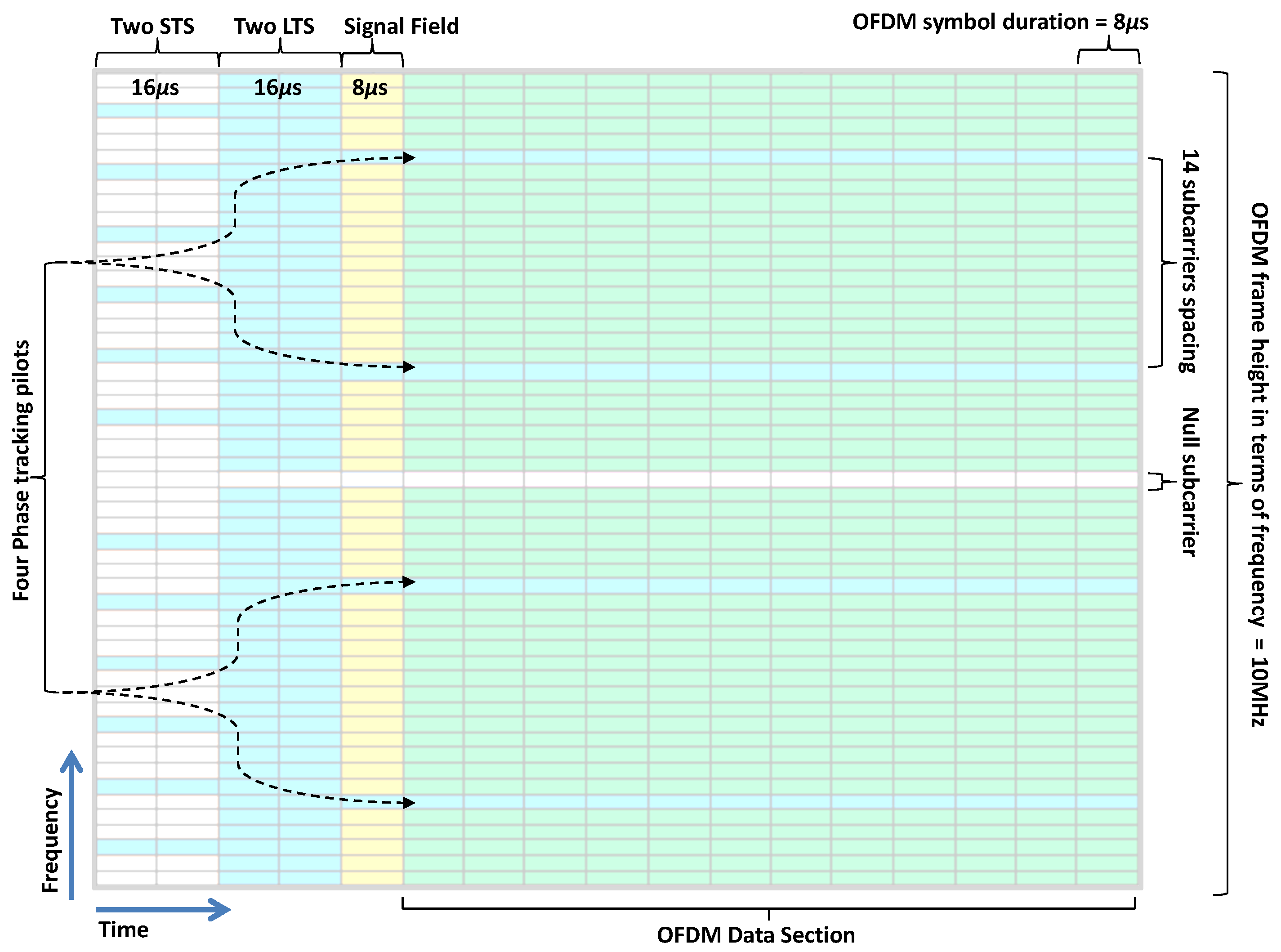
16]. In the IEEE 802.11p, channel estimation is performed by transmitting two predefined Long Training Symbols (LTSs) at the beginning of each packet. The channel is then estimated once for each packet, and this estimate is used to equalize the entire packet. IEEE 802.11p does not restrict the packet length. A channel estimate can quickly become less reliable for longer packets in V2V communications. Moreover, the IEEE 802.11p only allows the use of four pilot subcarriers (intended for residual frequency offset correction). These pilot subcarriers are not spaced closely enough to sample the variations of the channel in the frequency domain, which also contributes to performance degradation in V2V communications.
The main motivation behind the proposed scheme is to track the channel variations in time and frequency domain. In [
5], authors have investigated that channel estimation in the IEEE 802.11p standard can be improved by exploiting the correlation characteristics between the adjacent symbols of the orthogonal frequency-division multiplexing (OFDM) based data packet via constructing data pilots in the time domain. In this article, we have investigated that the adjacent subcarriers also have strong correlation characteristics in a data packet. We have employed these correlation characteristics in time and frequency domain to construct the reference data pilots for the channel estimation. In this way, an improved channel equalization can be achieved with a little complexity. The main contributions of this paper are listed here:
We have proposed an end-to-end channel estimation and equalization scheme for the IEEE 802.11p standard. It does not require modifications in the structure of the standard and keeps a balance between computational complexity and BER performance of the overall system.
In the channel estimation process, we have also utilized the correlation characteristics between adjacent subcarriers in the frequency domain, as well as between adjacent OFDM symbols in time domain.
The simulation results have demonstrated the performance improvement over CDP and spatial temporal-averaging (STA) schemes for V2V communications.
We have also presented an intuitive visualization of the V2V channel model which is used in the evaluation of the proposed scheme.
The paper is organized as follows.
Section 2 describes the current system model of the IEEE 802.11p transmitter and the channel.
Section 3 gives an overview of the current channel estimation schemes for the IEEE 802.11p.
Section 4 briefly describes the receiver and the integration of the proposed scheme.
Section 5 presents the simulation results and analysis of the proposed iCDP and
Section 6 discusses two important issues along with future work suggestions. Finally,
Section 7 draws the main conclusions derived from this work.
4. The Proposed Scheme
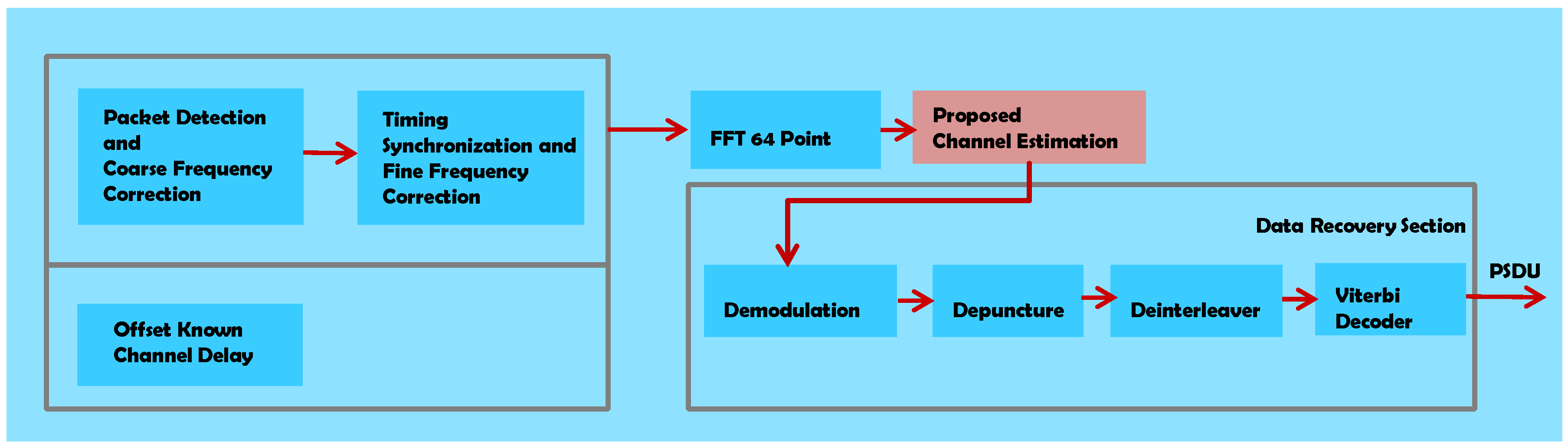
The block diagram of the receiver is shown in
Figure 3. The pink shaded box depicts the proposed channel estimator. It is placed after the 64 point FFT block.
Table 4 presents the timing parameters used in the simulation of the proposed scheme, and they are in accordance with Section 18 of the IEEE standard 802.11p [
1].
The timing synchronization and fine frequency correction are performed based on the output of packet detection and coarse frequency correction block. The detail about this block can be found in [
42].
Definition 2. Packet Detection: The process of detecting a packet based on the information in the received time domain signal , such as channel bandwidth. The output of this process is the offset, from the start of the received input waveform to the start of the detected preamble using auto-correlation.
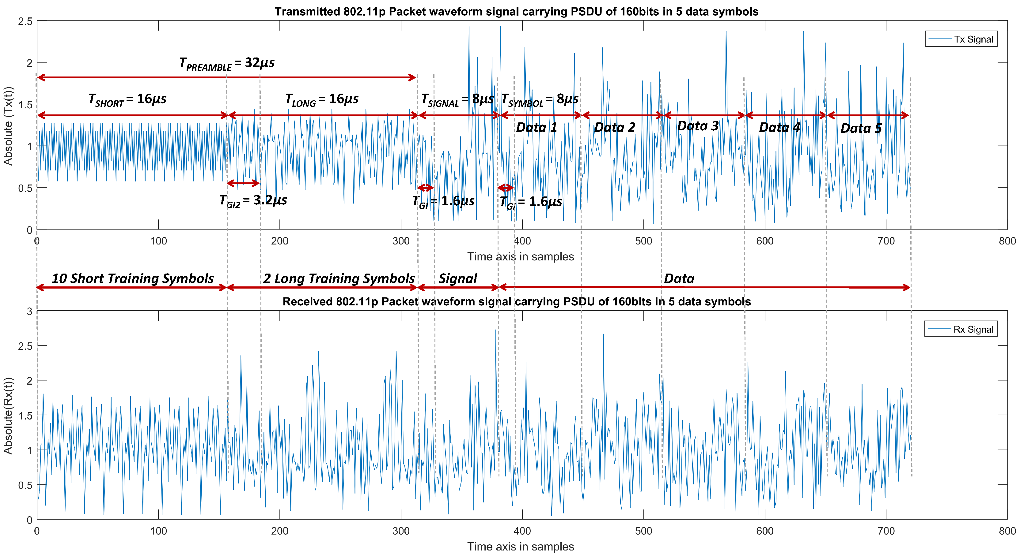
Figure 4 shows a single IEEE 802.11p packet waveform, where the upper part is the transmitted time domain signal and the lower part is the received time domain signal ready for channel estimation block. It should be noted that the transmitted time domain waveform
is a vector composed of complex numbers, therefore we have taken the absolute of the transmitted waveform i.e.,
and plotted in the upper part of
Figure 4.
Definition 3. Coarse Frequency correction: It is the correction in terms of frequency error which is estimated by utilizing the pre-known STS training field. The estimate contains the carrier frequency offset in Hertz. The short length of the periodic sequence in the STS allows coarse frequency offset estimation.
Similarly, the received waveform signal
that is modulated by channel [
28] and at
dB is drawn in the lower part of
Figure 4 as
. For the purpose of clarity, we have plotted only 5 data symbols.
Figure 4 also gives the detailed timing information in terms of parameters that are described in
Table 4. The output of the FFT block is
, which is the frequency domain representation of the received symbol at
kth subcarrier. In contrast to the CDP scheme, the proposed scheme also includes the 4 phase tracking pilots and therefore
k represents 52 subcarriers.
The proposed estimator updates the
ith symbol’s channel estimate by using the channel response
, obtained from the previous
symbol. The equalization process is given by Equation (
6).
Since
contains a total of 52 subcarriers. In order to construct 52 pilots, the
is divided into two groups of subcarriers, i.e., the data subcarriers group
and the phase tracking pilots subgroup
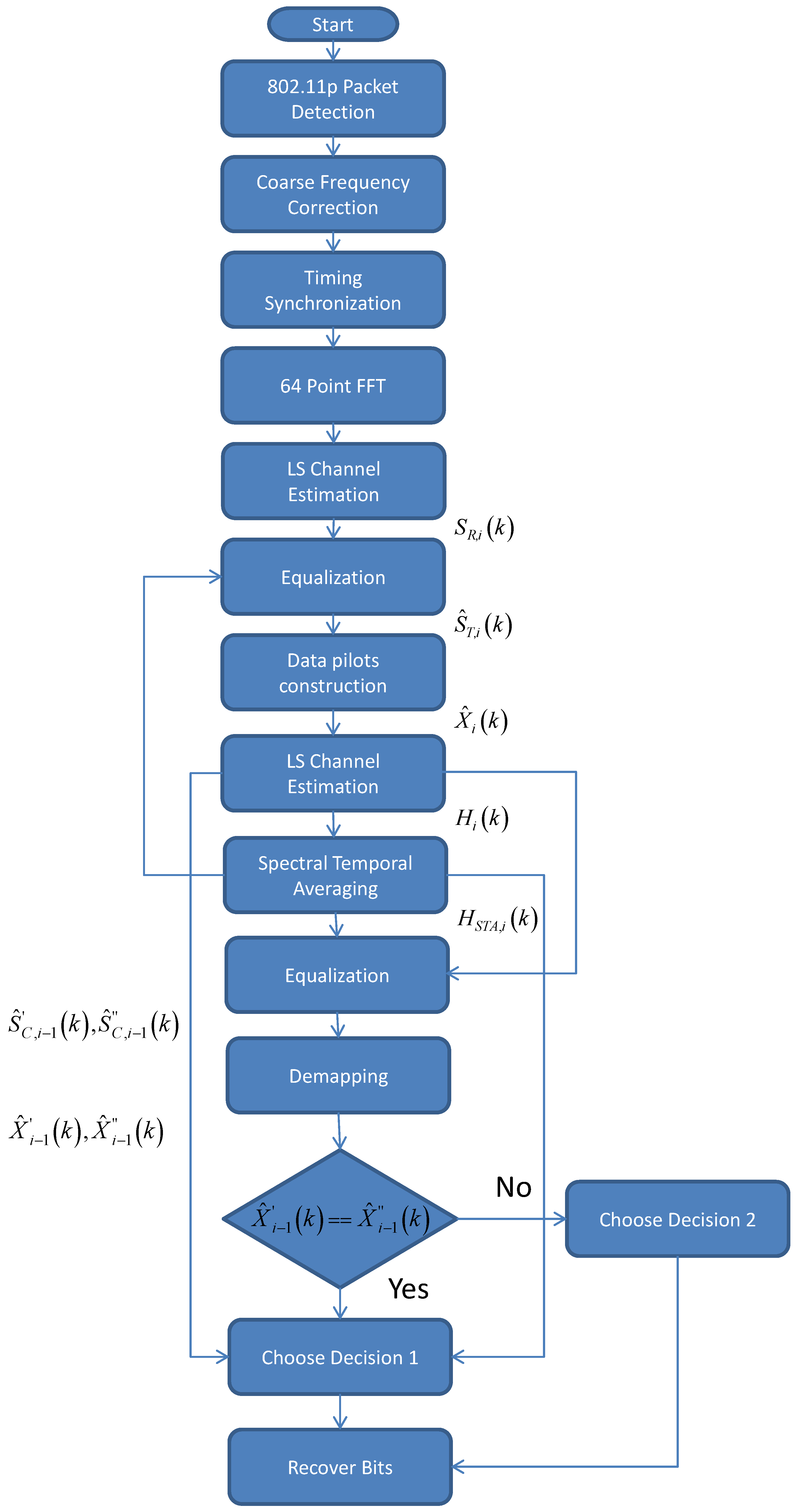
. These groups are then demodulated separately and then demapped to the respective constellation points to generate the two groups of pilots, i.e., one for the data subcarriers and the other for the phase tracking pilots. The reason behind the construction of the phase tracking pilots is to get more information for the comparison block. The process flow chart of the proposed channel estimator algorithm is shown in
Figure 5. It is clear from the process flowchart in
Figure 5 that the time domain signal in
Figure 4 is now converted to the frequency domain by taking the 64 points FFT. Then the LS estimation is performed on this signal using Equation (
1). As stated earlier, the next task is to perform the equalization to get a rough estimate of the transmitted LTS. The initial Data pilots are created and then again LS estimation is performed which is based on the constructed data pilots.
Since the adjacent subcarriers to the phase tracking pilots have a higher correlation with them, so the constructed phase tracking pilots and the originally known phase tracking pilots are compared to decide the channel response in those regions, which helps in improving the accuracy of the overall system. In the CDP estimation scheme, the assistance of demapping is used to partially alleviate the impact of noise from the other interferences. Then, the remaining error is further reduced by exploiting the correlation characteristics of the channel for the two adjacent symbols. The constructed data pilot
in [
5] are then employed to obtain the
ith data symbol’s channel response by using the Equation (
3). We further investigated that even though
is a relatively accurate estimate of the channel response, however, it is can be improved by exploiting the high correlation characteristics of the channel. Therefore,
is used to equalize
in Equation (
7).
Again, the
is then equalized by
, i.e., the previous symbol’s estimated CR, which has been used before in Equation (
6). In order to make a comparison,
is also equalized by the
and the resulting equalized
is given by Equation (
8).
The one to one comparison of
and
is made by appropriately demapping them to their respective constellation points
and
. The proposed demapping process starts by using constellation demodulation of
and
, using the information from the standard IEEE 802.11 modulation coding scheme (MCS) table. Let us take the case of
= 2, so that after the demodulation the
is now represented by
and
is represented by
. For this particular configuration,
can take four different values represented by
Equation (
9) to Equation (
12).
Let say
,
,
, and
represent the values
,
,
, and
respectively. In order to choose the best value, we need to take the absolute difference of
(where
n can take any value from 1 to 4) from
,
,
, and
to get
,
,
, and
as shown in Equation (
13).
Then the argument or index of the minimum value from
is selected as shown in Equation (
14).
The prediction of the actual value of
and similarly that of
can be found from Equation (
15).
If
, it means that the
subcarrier’s
is not valid and the assumption is made that
. Additionally, if the
, then it can be assumed that
, which is indicated as
1 in
Figure 5. We argue that the two adjacent data symbols have high correlation in frequency as well. Therefore if
, it indicates that the
kth subcarrier’s
, which demapped after Equation (
6) is incorrect and we should define that
, i.e., the previous symbol’s estimated CR. It is indicated as Decision 2 in
Figure 5. Moreover, in contrast to the CDP scheme where otherwise, if
then
. We argue that the superior performance over CDP scheme can be obtained by taking into consideration
obtained previously from Equations (3) and (5) through the Equation (
16).
where
is the proposed channel estimate. The next section evaluates the proposed estimator over the severe channel conditions of [
28] and also provides comparisons with the closely related schemes. Let us assume that
represents the absolute of the estimated channel.
5. Simulation Results and Analysis
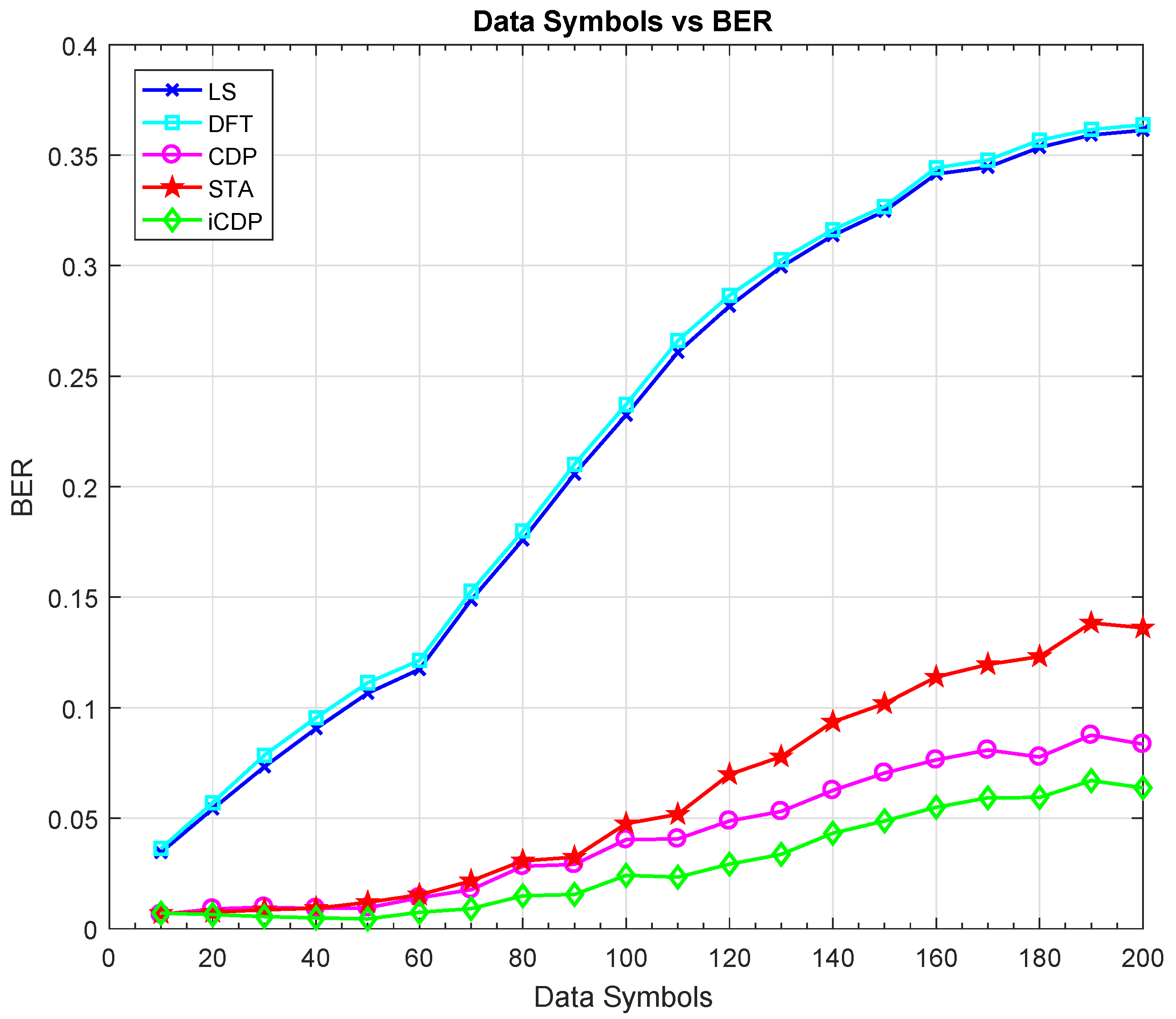
The simulation platform used in this article is Matlab 2016b. The BER simulation results of different configurations are presented in this section. We have compared the proposed iCDP scheme with LS, DFT, STA, and CDP schemes. The value of parameters
and
is set to 2 for the optimal performance of the STA scheme as discussed in [
36]. The performance of IEEE 802.11p is analyzed under the different length of packets i.e., from 10, 20, 30, and up to 200 OFDM data symbols. The simulation results reveal that LS and DFT channel estimation schemes have higher BER values, whereas STA, CDP, and iCDP are comparatively better under all symbol lengths as shown in
Figure 6.
The value of maximum Doppler shift is set to 1200 Hz for the HIPERLAN-E channel and the modulation coding scheme is
. It is also obvious from
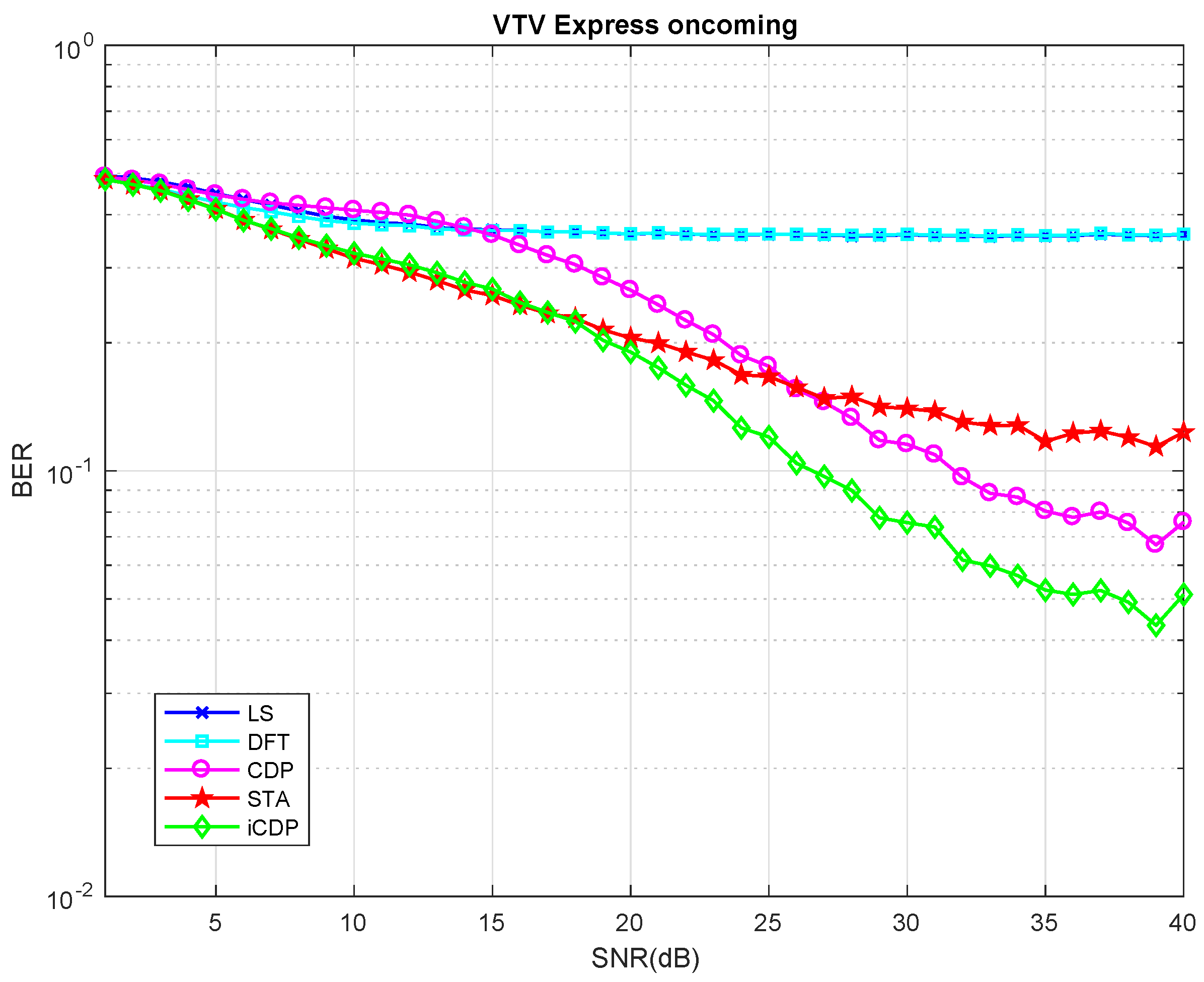
Figure 6 that the BER values for STA, CDP, and iCDP remain almost same for the 10 and 20 data symbol lengths, however, as the length increases, iCDP tends to perform better than STA and CDP. The next test is performed for the VTV express oncoming channel model as shown in
Figure 7. It is also clear from the results that under the lower SNR regions the STA scheme performs better than CDP scheme, however, the proposed iCDP scheme performs better than CDP scheme and nearly similar to the STA scheme.
In the higher SNR regime, the CDP scheme outperforms the STA scheme. This is due to the fact that under the lower SNR the noise and interferences are strong enough to move the to the incorrect locations, which results in demapping of to the incorrect constellation points.
The increase in SNR reduces these incorrect demappings and the CDP scheme performs better in this regime. In contrast to the CDP scheme, the iCDP is inherently SNR aware. This is due to the reason that the construction of data pilots is followed by LS channel Estimation and STA equalization, which reduces the error demapping probability of to the constellation points. The results show that the STA and iCDP schemes perform equally well as compared to CDP up to the SNR value of 18 dB. On the other hand, CDP and iCDP perform better than STA from the SNR greater than 26 dB. The iCDP overall performs better than the CDP scheme. Due to the page limit, the result of the rest of the 5 channel models are skipped and the next results are for the HIPERLAN-E channel model.
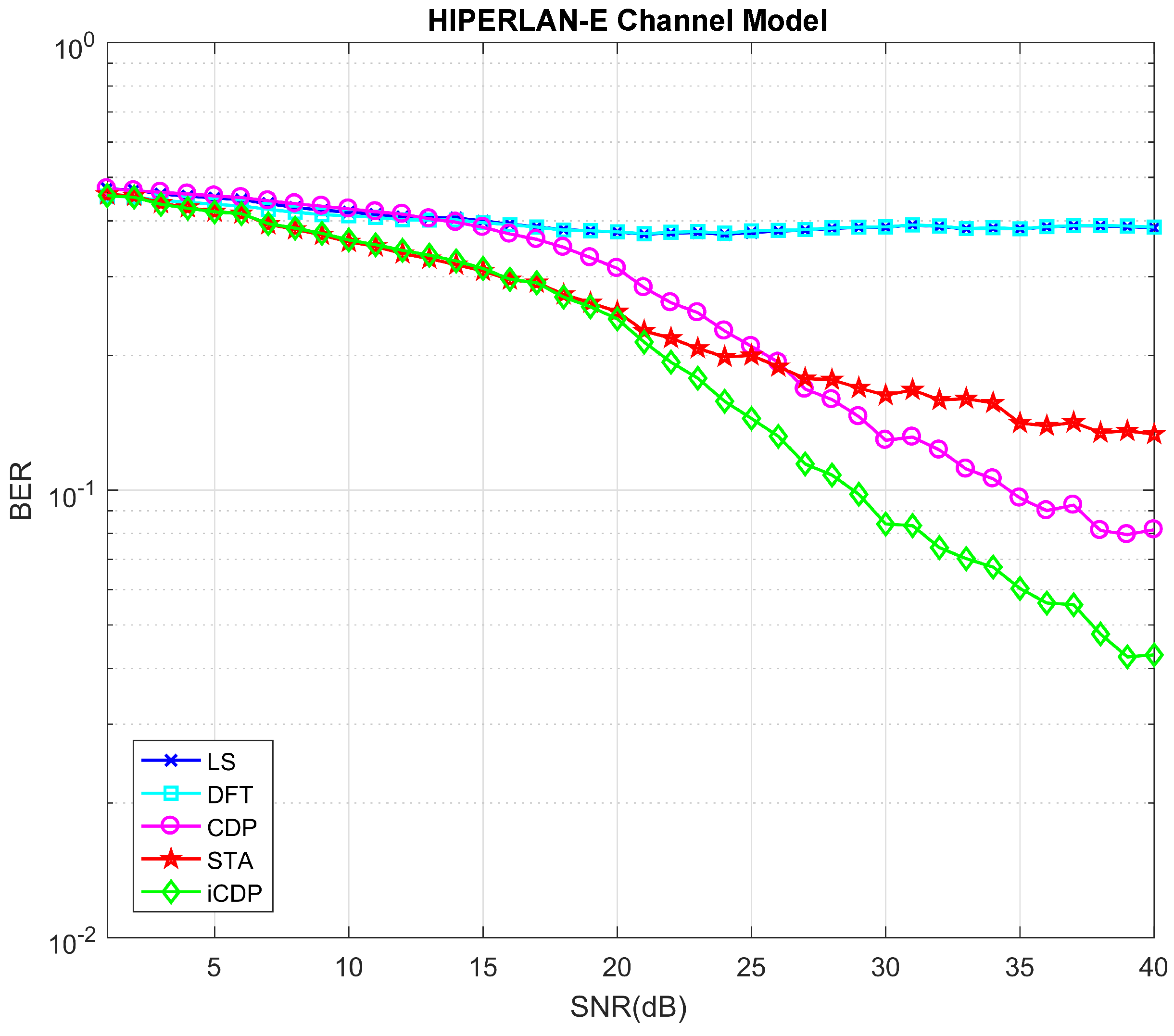
Under urban traffic scenario the number of buildings and vehicles increases, hence scattering and reflection of the transmitted signals also increase. This phenomenon leads to an increase in the number of multi-path fading. The HIPERLAN-E channel model has a total of 18 multi-paths.
Figure 8 shows the result of the BER performance curves of different schemes for this channel model. The results show that the STA and iCDP schemes perform equally well as compare to CDP up to the SNR value of 20 dB. On the other hand, CDP and iCDP perform better than STA from the SNR greater than 22 dB.
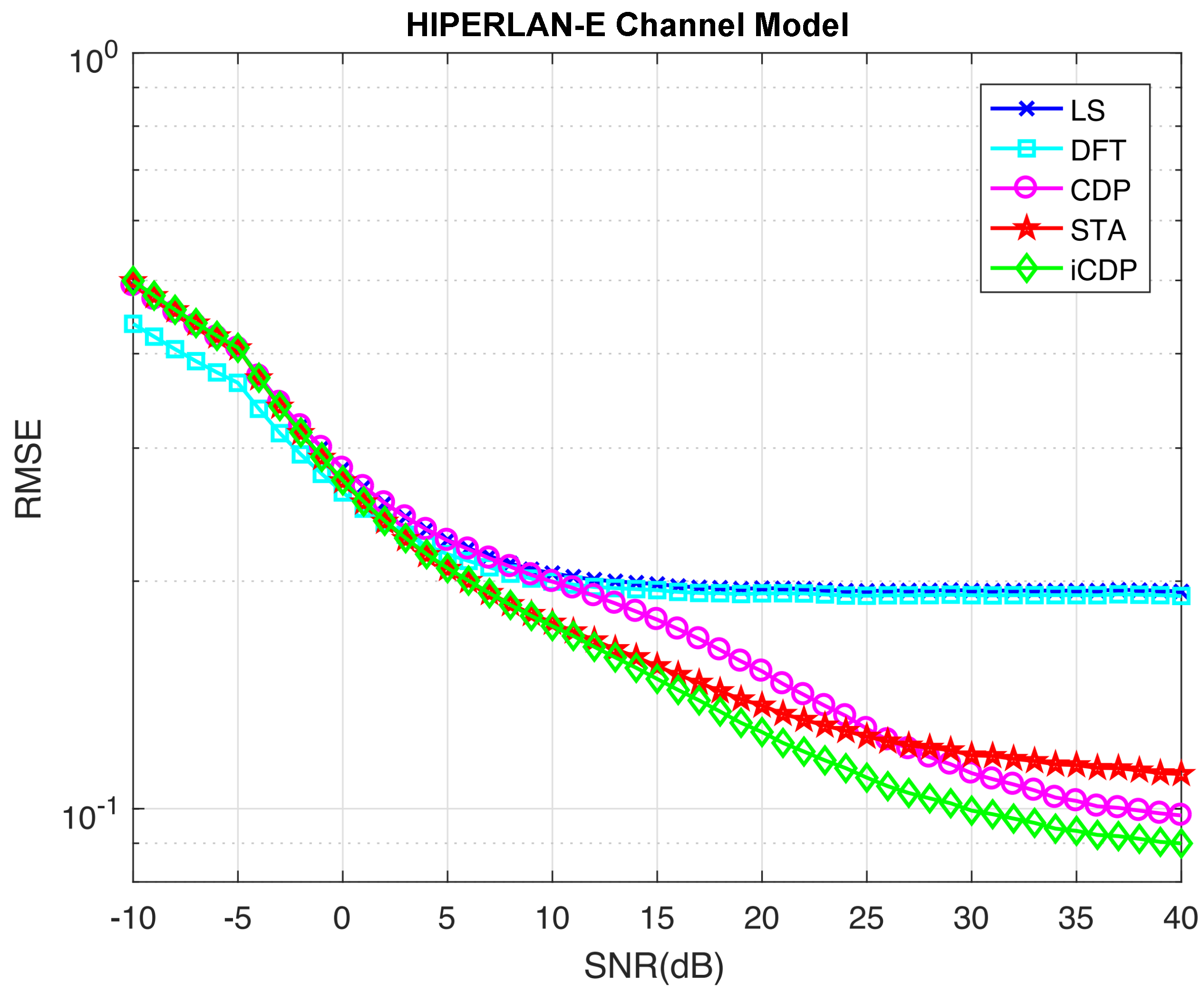
The performance comparison in terms of RMSE is shown in
Figure 9. The method to obtain RSME is described in [
6]. It is clear that at an SNR of −10 dB, the DFT scheme performs better than others. The RMSE value DFT scheme is 0.4381 at −10 dB, while the other schemes have roughly the same value of 0.4994. It is due to the fact that DFT ignores the noise-containing coefficients of the time domain channel response. However, the RMSE performance of DFT degrades as the SNR becomes bigger. The iCDP and STA schemes perform almost similar till the value of SNR equal to 8 dB. However, CDP scheme performs similarly to LS scheme until SNR equal to 8 dB. The RMSE values obtained at SNR equal to 8 dB for LS, DFT, CDP, STA, and iCDP are: 0.2111, 0.2046, 0.209, 0.1865, and 0.1860 respectively. If we go on further at the point where SNR is 26 dB, then the STA and CDP schemes have roughly similar RMSE value of 0.1227 and the iCDP scheme has a value of 0.1071. The RMSE values of DFT and LS schemes are 0.1916 and 0.1943 respectively. Finally, at an SNR of 40 dB, the RSME value of iCDP is 0.0899 and corresponding RMSE values for CDP and STA are 0.9796 and 0.1112 respectively. The RMSE for LS and DFT seems saturated at roughly 0.1916 with no further improvement in performance. This result demonstrates the performance improvement of the proposed scheme over DFT/LS, STA, and CDP schemes with the RMSE percentage differences of 72.3%, 21.1%, and 8.5% respectively at SNR of 40 dB.
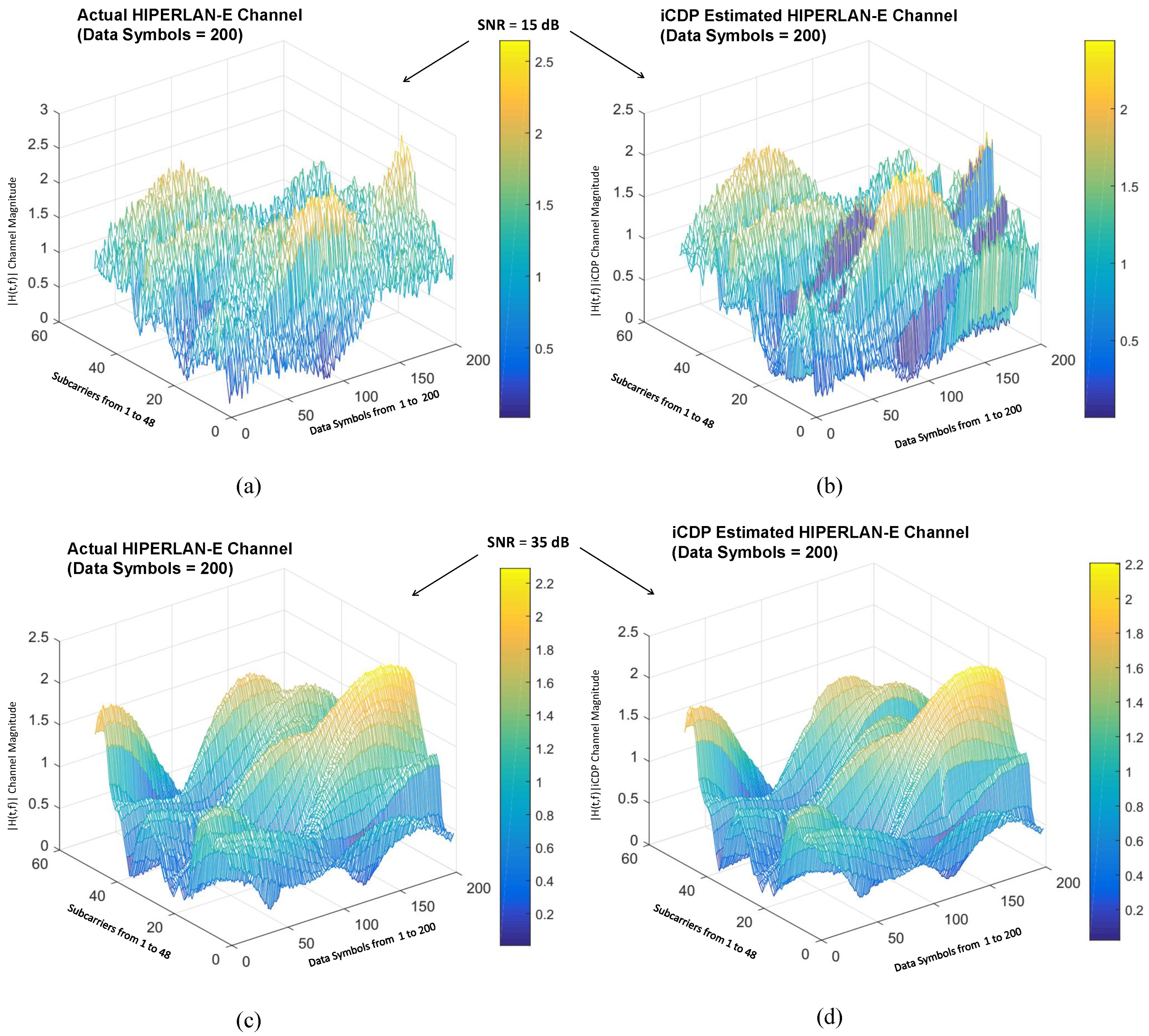
It is equally important to visualize the 3-dimensional image of the actual HIPERLAN-E channel and its estimation by the proposed iCDP scheme to show that it tracks the channel in time and frequency domain for the different SNR values.
Figure 10 shows the effect of lower and higher SNR on the HIPERLAN-E channel model.
Figure 10a shows the actual channel conditions at under
, data symbols = 200, and SNR = 15 dB.
Figure 10b shows the estimation of the actual channel in
Figure 10a through the proposed scheme. On the other hand,
Figure 10c shows another channel conditions at SNR = 35 dB and
Figure 10d shows its estimation through the proposed scheme. It is evident from
Figure 9 that at lower SNR, the correlation among the data symbols and frequency subcarriers suffers due to the randomness of the noise. The proposed scheme performs relatively better than CDP under lower SNRs because it constructs the data pilots after taking into consideration the front and previous data symbol in time domain and front and previous frequency carrier in the frequency domain.
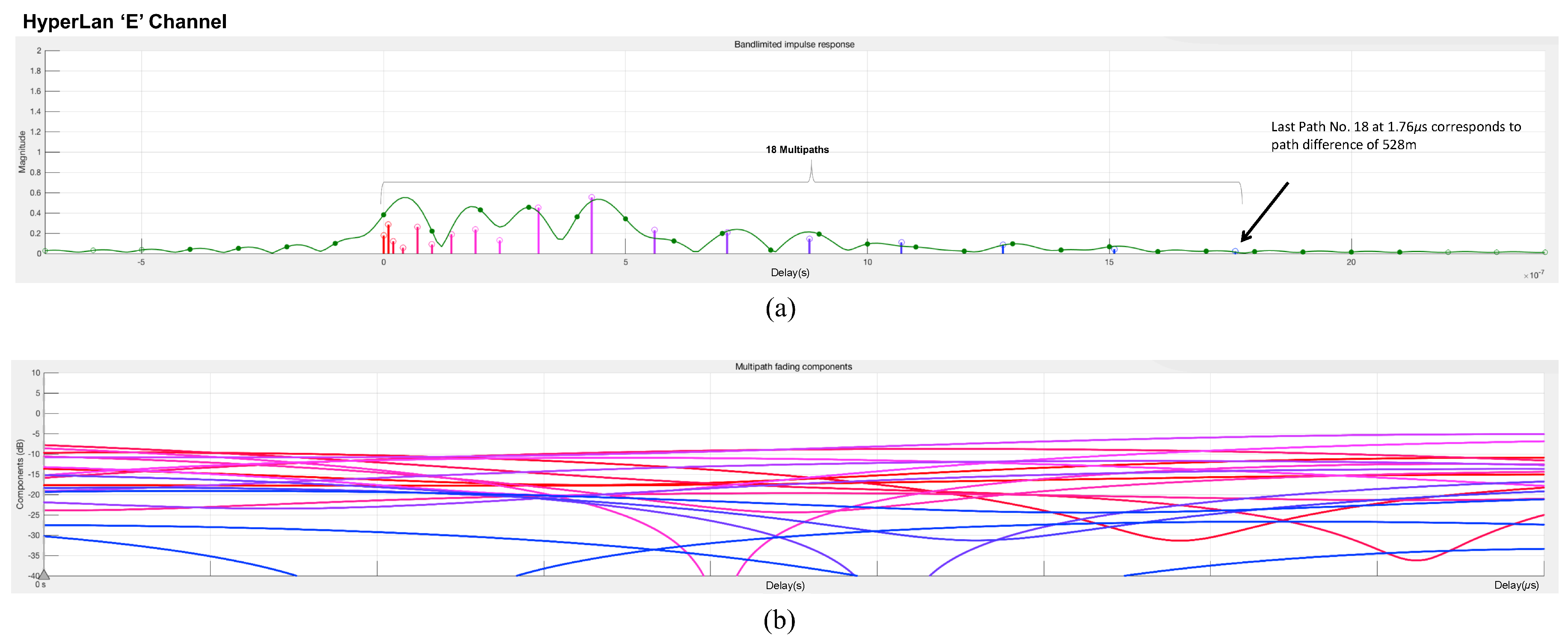
Figure 11 shows the multipath components of the HIPERLAN-E channel used in the simulation of the proposed scheme. The bandlimited impulse response in
Figure 11a shows 18 different paths that are arriving at the receiver vehicle with different amplitudes and delays.
Figure 11b shows the contribution of these components with the passage of time up to 850
s. The delay of the first path is set to 0
s. For subsequent paths, a 1
s delay corresponds to a 300 m difference in path length. In vehicular communication, the multipath environments have reflected paths that can be up to several kilometers longer than the shortest path. With the path delays specified above, the last path is 528 m longer than the shortest path, and thus arrives 1.76
s later which is also obvious from the specifications in
Table 2. The path delays and path gains specify the channel’s average delay profile.
Typically, the average path gains decay exponentially with delay (i.e., the dB values decay linearly), but the specific delay profile depends on the propagation environment. In the delay profile specified in
Figure 11, we assumed the specifications of
Table 2 HIPERLAN-E channel model.
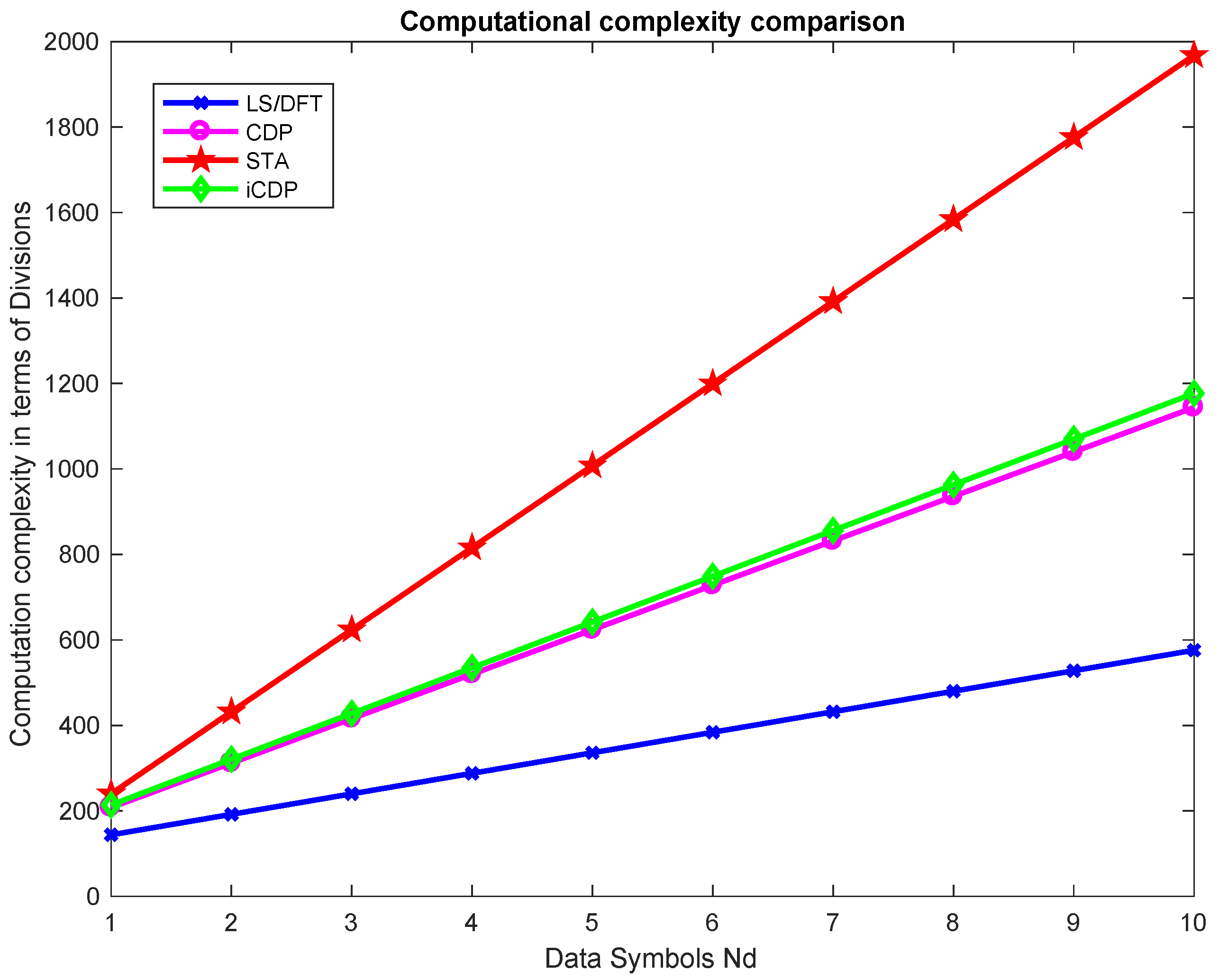
Computational Complexity
Figure 12 shows the comparison of computation complexity in terms of the number of additions, as a function of the number of data symbols
.
Table 5 summarizes the comparison of the computation complexity of different scheme in terms of divisions, multiplications, additions, and subtractions.
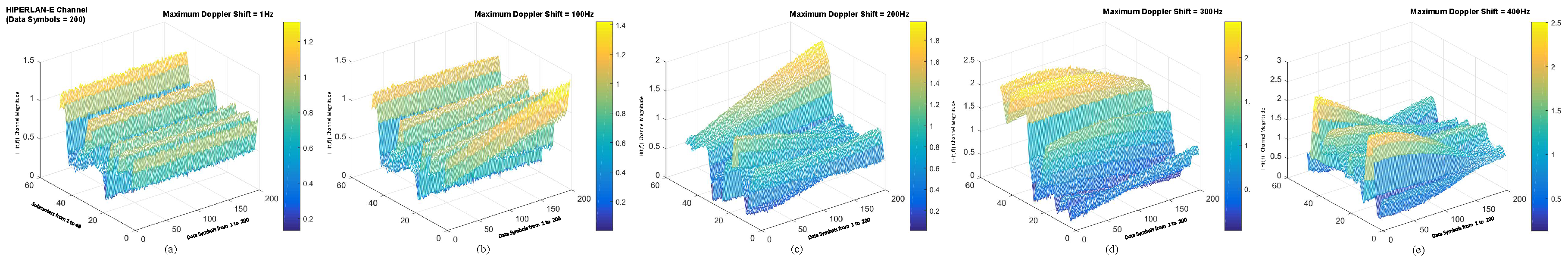
The higher Doppler shift causes stronger variation in the time domain as well. It is therefore essential to visualize how the value of
effects the channel conditions in time domain or along the length of data symbols.
Figure 13 shows this effect for different values of
i.e., 1, 100, 200, 300, and 400 Hz.
The impact of these values on the channel conditions is shown in
Figure 13a–e. It is interesting to notice that at a very low value of
= 1 Hz, the channel remains almost invariant in the time axis. Then the variations become larger as the value of
increases.


