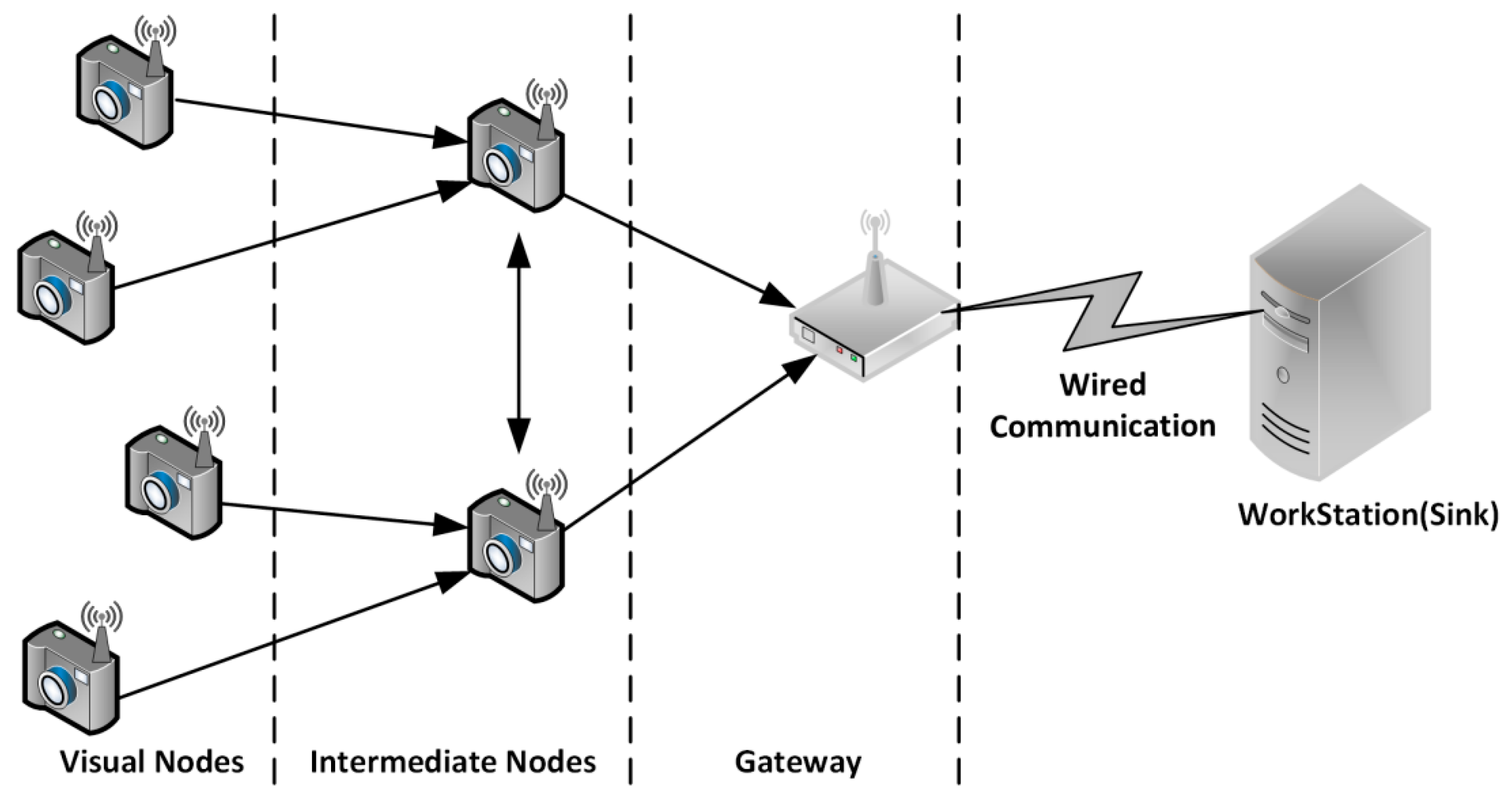
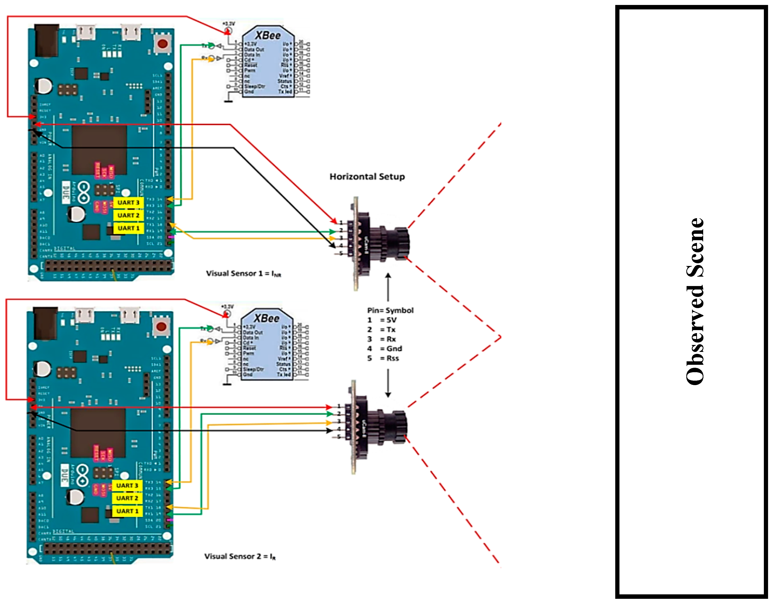
A VSN platform primarily consists of hardware and software components. The hardware component includes the camera, processing unit, and transmission module that work together to create a visual node that is capable of capturing and sending the data to the workstation for further processing. Whereas the software component includes image acquisition, encoding process, and communication protocol that helps to compress and packetize the data before transmission. As shown in
Figure 1 is an example of how devices in VSN are typically connected. The development of the platform also aims to create a simple, flexible, and low-cost VSN platform integrated with energy efficient compression.
Details of the hardware and software components used to implement the proposed scheme are provided in the following subsections.
3.1.1. Hardware Components
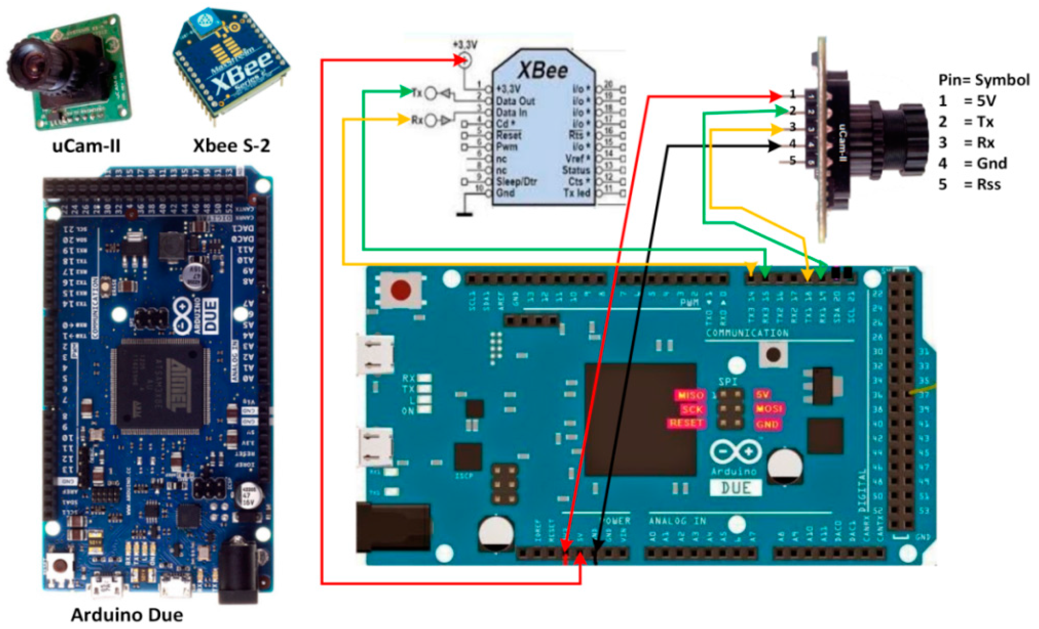
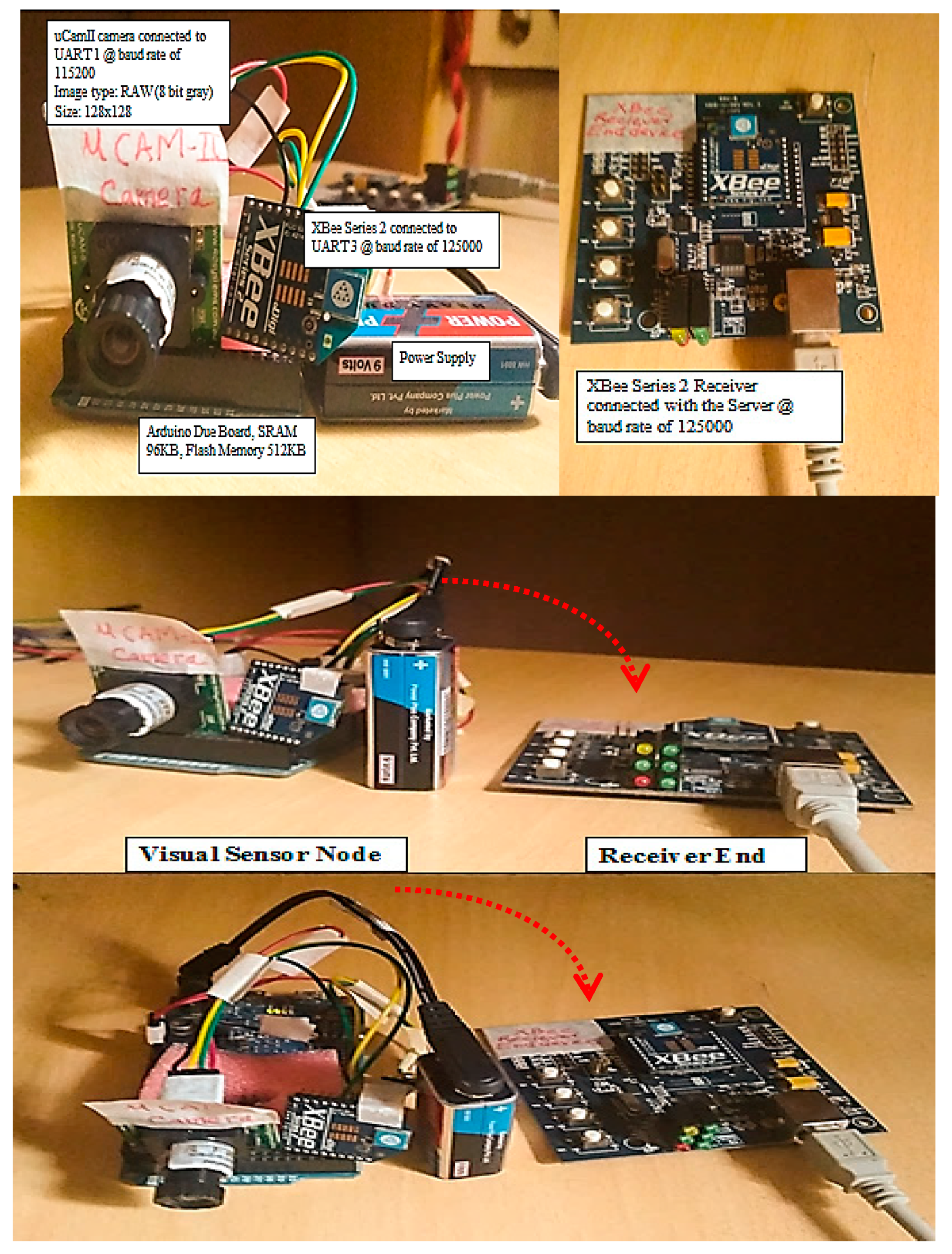
As shown in
Figure 2, a visual node that consists of an Arduino Due board [
28], a CMOS uCAM-II camera [
29], and an XBee transmission module [
30].
1. Arduino Due Board
Although there are several other microcontrollers available, Arduino is a low-cost card-size board that offers sufficient processing power and memory for simple computation tasks. Moreover, its functionalities can be extended by connecting to many other peripherals (or shields), the code developed for one model can be reprogrammed and run on other Arduino board with minimum modifications. In the development of the proposed BCS visual node, an Arduino Due board [
28] is selected. It is equipped with an Atmel SAM3X8E ARM Cortex-M3 microcontroller running at 84 MHz, 96 KB of SRAM memory, and 512 KB of flash memory. In addition to this, it also comes with several UART interfaces that can be used to communicate with other external components. The reason of selecting Due over other Arduino boards is that it uses less energy (runs at 3.3 V), higher computing performance (clock speed of 84 MHz), and has more SRAM and flash memory. Overall, it is difficult to implement the image processing task on other Arduino boards due to the limited amount of memory.
2. uCAM-II CMOS Camera
Among the many low-power, low-cost CMOS cameras [
32,
33,
34,
35,
36], the uCAM-II by 4D schemes is selected [
29] for the development of the BCS visual node. Unlike the other available cameras that only provide images in JPEG format, the uCAM-II is capable of providing images in both raw and jpeg formats. Furthermore, uCAM-II can capture images at resolution ranges from 80 × 60 to 640 × 480. Moreover, the uCAM-II is also compatible with lenses of different viewing angles. These include the standard 56-degree lens that comes together with uCAM-II, as well as the 76-degree lens and the 116-degree lens can be purchased as additional components. It operates on normal 5V DC supply, and no external DRAM is required for storing the images. The uCAM-II is connected to the Arduino Due board through one of the UART interfaces at 115,200 bauds.
3. XBee Wireless Module
Wireless communication between the visual node and the server is performed by using an XBee module. It can send and receive data via the 2.4 GHz or 900 MHz band at relatively low power. They can be used to set up a simple point-to-point link by using the transparent mode or to form a complex self-healing network that spread over a large area when using the API mode [
37]. For the development of the BCS visual node, the XBee module is configured to operate in the API mode. In this case, the visual data is enclosed in a packet before transmission takes place. The XBee module is connected to the Arduino Due board through another UART interface. However, 125,000 bauds are used because the communication between the XBee module and the Due board is not reliable at 115,200 bauds given the Due’s clock frequency of 84 MHz [
37].
3.1.2. Software Components
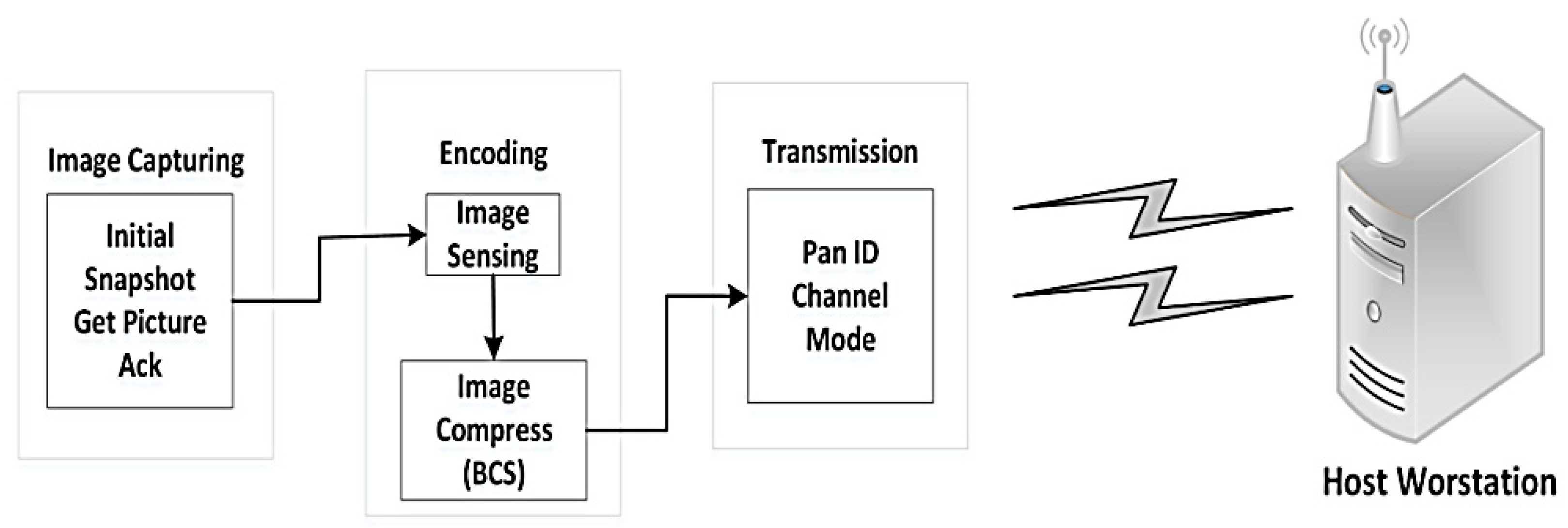
In this context, the software architecture is built using modular design. As shown in
Figure 3, the platform consists of data preprocessing in the sensor side, control protocol during the transmission, and stream management in the server. We will summarize several key components in the rest of this section.
1. Image Capture
In our implementation, we capture an 8-bit grayscale raw image and store the image data in the Arduino flash memory for further processing. As Arduino Due has a larger flash memory than SRAM, it is better first to store the large image data into flash memory using PRGMEM variable modifier and then read the data from flash memory back into SRAM using a block-by-block approach.
To start the communication process, a connection between the host and the uCAM-II must be established. As shown in
Figure 4, this is started by synchronizing the host with the uCAM-II via SYNC command. The SYNC command is sent periodically to awake the camera from sleep state if no commands have been sent. If communications are occurring between the host and the camera, the camera will stay awake. The host sends the SYNC command continuously until an acknowledgment (ACK) and SYNC command is received from the uCAM-II. A maximum of 60 SYNC command can be sent to awake the module. If the module does not respond after 60 SYNC commands, it is restarted, and the same actions are performed again. Usually, up to 25 to 60 SYNC commands may be necessary before the module will respond. After the host receives the response, it should reply with the ACK command to confirm the synchronization process.
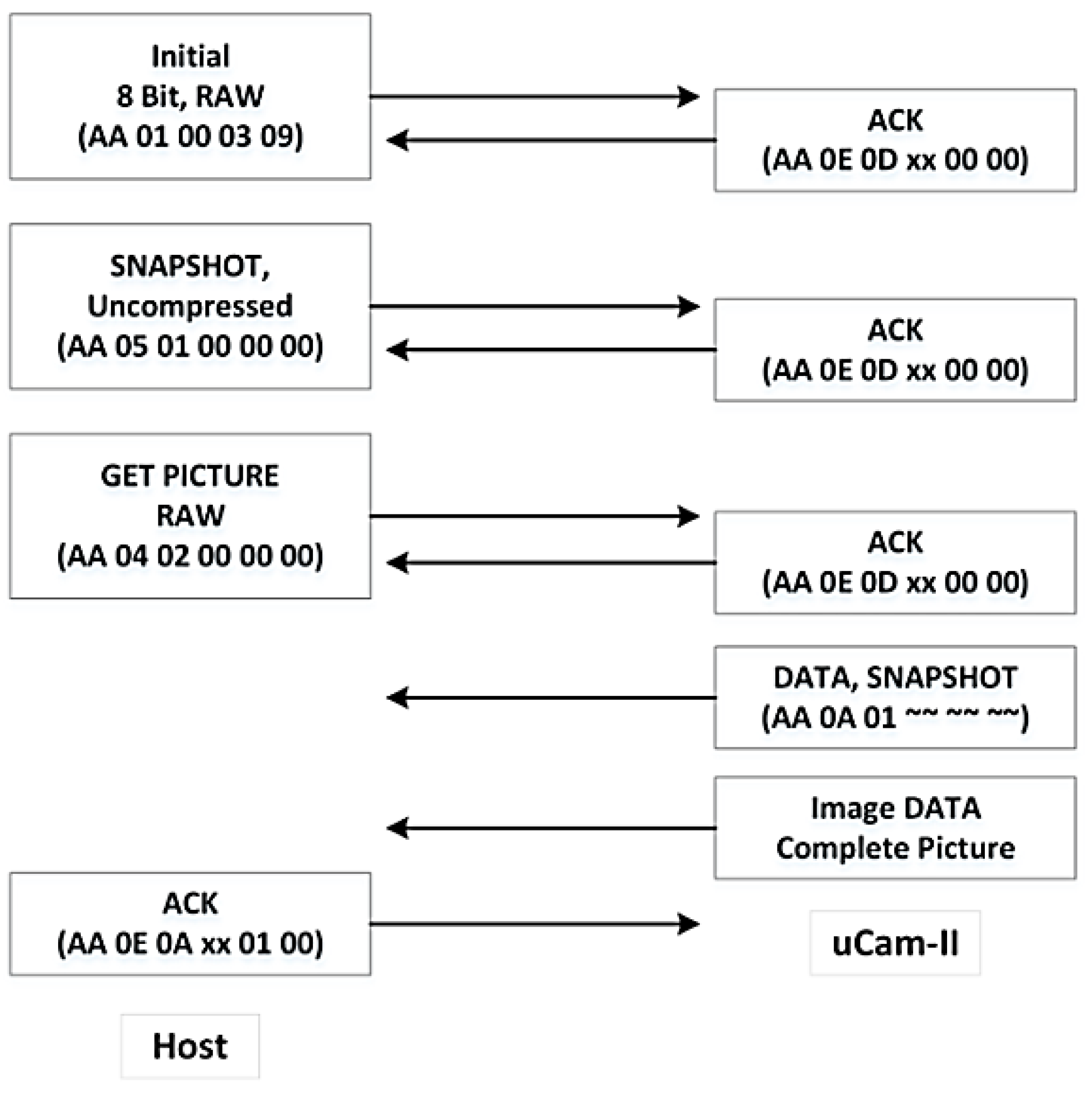
After the communication link is established, uCAM-II is ready to capture images. In order to capture a raw image, the following commands have to be sent from the host to the uCAM-II.
INITIAL is first used to configure the image size and image format.
SNAPSHOT is to instruct uCAM-II to capture an image and store it in the buffer.
GET PICTURE is used to request an image from the uCAM-II.
ACK is sent to indicate the end of the last operation.
The overall process of capturing an 8-bit grayscale raw image with a resolution of 128 × 128 raw is shown in
Figure 5. This resolution is selected because Arduino Due has limited SRAM of 96 KB.
2. Encoding Process
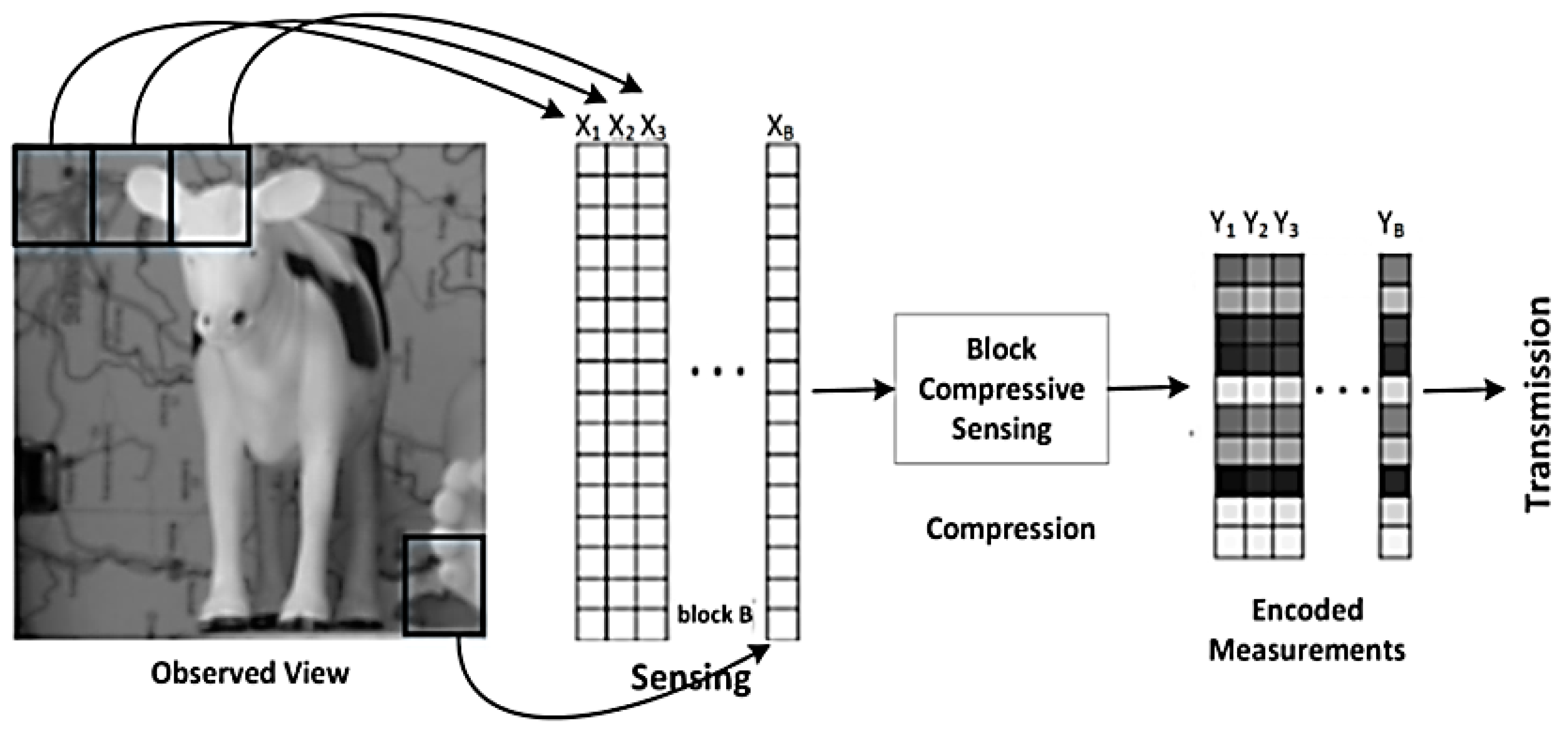
The image obtained from uCAM-II is first stored into the flash memory. The BCS is applied to encode the image on a block-by-block basis. The encoding process can be divided into two parts, namely image sensing, and image compression as shown in
Figure 6.
In the first part, the raw image of resolution 128 × 128 is first divided into small 16 × 16 independent blocks, and each block is rearranged into a vector with 256-pixel values. This produces a matrix of size 256 × 64, and this is denoted as the sensed measurement, I. Next, I is sampled by random measurement matrix Φ. The measurement matrix Φ used in the JMD scheme is a constrained structure (block diagonal) matrix that is incoherent with any sparsity basis with a very high prospect. This also reduces the memory required to store the measurements when it is implemented as a dense matrix. The size of the measurement matrix Φ is determined based on the block size and sampling rate. For example, if the block size is 16 × 16 and the sampling rate is 0.2, then the Φ generated is of size 51 × 256. Then Φ is multiplied with I to obtain the encoded measurement matrix Y. All the encoded measurement will then be transmitted to the server via the XBee module. However, before transmission, the encoded measurements are quantize using uniform quantization. Each measurement value is converted to a signed 16-bit binary vector. From our analysis, the measurement value can exceed the range of −128 to +128. Hence, it is not sufficient to fit the value into a signed 8-bit binary vector.
3. Wireless Communication
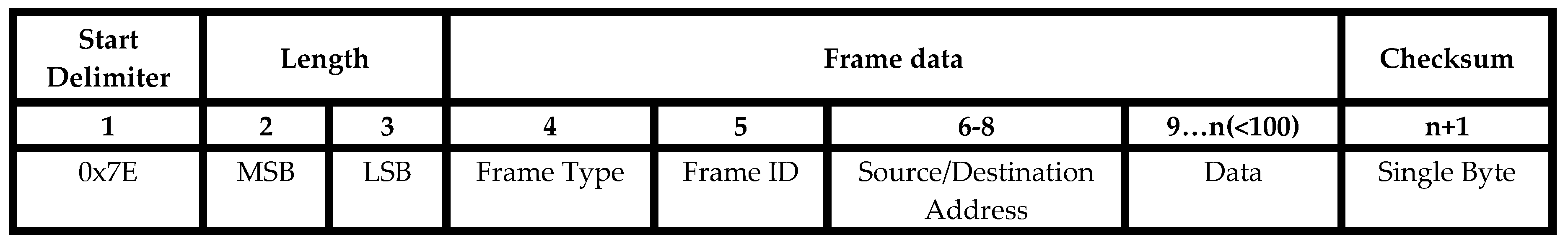
Two Series-2 XBee modules are used. One is connected to the Arduino Due, and the other is connected to the server. The former is configured as the end device that is in charge of sending data, whereas the latter is configured as a coordinator that is in charge of setting up the network and receiving data. It is also necessary to ensure that they are operating under the same PAN ID and channel number. All these parameters have to be configured before forming a wireless network. The API mode is used over AT mode to emulate the transmission pattern of a VSN. The API mode is designed to transmit highly structured data in a fast, predictable, and reliable way. The XBee modules were configured in API mode, having a baud rate of 125,000, data bits of 8, no parity bits, and 1 stop bit. In API mode, the input data will be packetized into many API frames before transmit within the wireless network. The API frame structure is shown in
Figure 7 [
37].
In every API frame, the first byte is a start delimiter that is used to indicate the beginning of each API frame. The value is always 0 × 7E allowing easy detection of a new incoming frame. The next field indicates the length of the frame. The length is of 16 bits value and is divided into MSB (most significant bits) and LSB (least significant bits). After the length is the frame type, frame ID, source or destination address and the payload (data). The frame type indicates how the information is organized in the data field. The frame ID is used to enable a form of acknowledgment that shows the result of the transmission. The source or destination address is a 64-bit value that means either the source or the destination of the packet. The data field contains the information to be transmitted and is dependent on the frame type.
The value in each field may vary according to transmit or receive the request. For transmit request the frame type, frame ID, 64-bits source or destination address values are 0 × 10, 0 × 01, 0 × 000000000000FFFF (destination address) respectively whereas, for receive request the values are 0 × 91, 0 × 00, 0 × FFFFFFFFFFFFFFFF (source address) respectively. The last field of the API frame is the checksum that is used to test the data integrity. The checksum is calculated by first adding all the bytes in the frame excluding the start delimiter and length, then subtract the lowest 8 bits of the result from 0 × FF.
• At the Coordinator End:
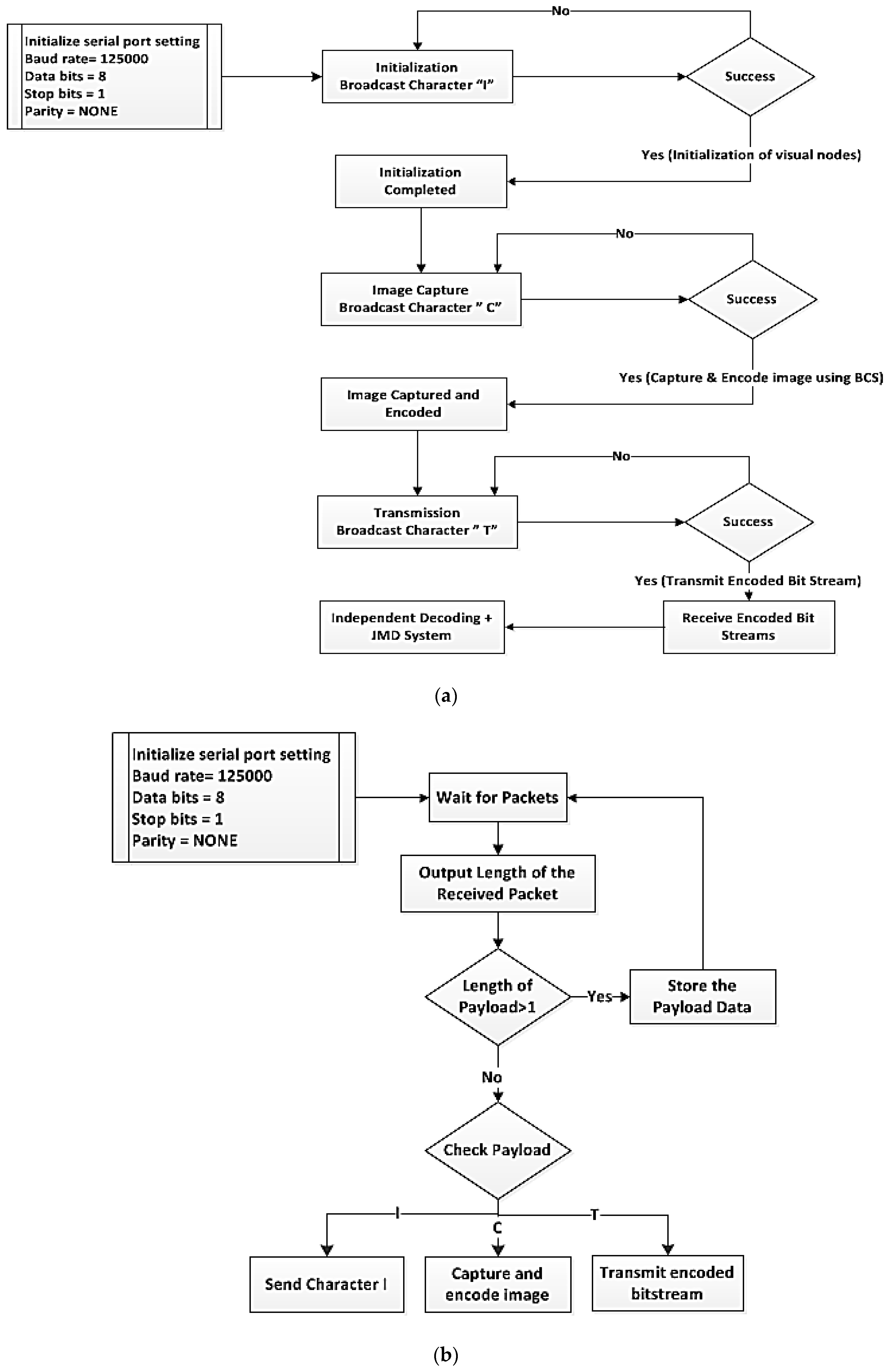
The server is connected to the XBee module (the coordinator) for receiving data transmitted from the visual nodes. Once the coordinator has set up the network, other end devices (visual nodes) will be able to join the network automatically. The communication between the coordinator and the visual node is illustrated in
Figure 8a.
- ○
Initially, the server will broadcast a packet containing an ‘I’ (Initialization) character via the coordinator to all the visual nodes. This step is to define the number of visual nodes in the network (i.e., to identify the number of images that are to be received). If the end device successfully receives the packet, then a ‘Yes’ signal is generated, and an acknowledgment is sent back to the coordinate. If the acknowledgment is not received by the coordinator from the end device for some time, the packet is unsuccessfully and is resent. This initialization step helps to determine the number of visual nodes in the network and to know the number of images that are going to be received. This is followed by broadcasting two more packets containing character C (capturing) and T (transmission) in their respective order.
- ○
Once the initialization is completed, the coordinator will broadcast the next signal containing a ‘C’ character. The ‘C’ character will update the visual nodes to capture and encode the image data with the BCS scheme.
- ○
Similarly, after receiving an acknowledgment from the end device, another signal comprising of ‘T’ character is sent to each visual node in the network. As soon as the visual node receives the ‘T’ character, it will start to send the encoded stream to the coordinator (server).
- ○
After the server has received the encoded stream, the stream will be decoded to recover the captured images by using independent BCS with JMD scheme. As multiple images (due to more than one visual node) will be received at the coordinator (server) end, it is essential to separate the data transmitted by the different visual node. It is done by referring to the automatically embedded source address in the transmitted packet.
- ○
Finally, the process described above is repeated for the next transmission cycle.
• At the End Device:
The XBee module is connected to the Arduino board through a serial port to serve as an end device (visual node). The end device will automatically connect to the initially established network by the coordinator. The communication between the end devices (visual node) and the coordinator is illustrated in
Figure 8b.
- ○
The visual node is always looking for signal (Packet) transmitted from the coordinator (server).
- ○
Once a packet (API frame) is successfully received, the visual node will process the information acquired from the packet. If the received packet contains an I; the same packet will be transmitted back to the server for acknowledgment purpose. It is from the initialization as discussed in the above section.
- ○
If the received packet contains ‘C’, the node will capture and encode the images using BCS. The reason for doing this is to synchronize the image capturing process of different visual nodes. This is to ensure that the images are captured at approximately the same time to ensure maximum correlation. Furthermore, this also allows the server to control when the capturing should take place.
- ○
Once a packet that contains a ‘T’ is received, the visual node will wait for packets (encoded measurements) to packetize the encoded measurements into numbers of API frame, and each frame has a payload size of 72 bytes. All the data will be continuously transmitted to the server until there is no more data to transfer. Then, a packet that carries a value of zero is sent. The purpose of this frame is to inform the server that the previous packet was the end.
3.1.3. Theoretical Basics of Compressive Sensing
CS states that a signal that is sparse in some transform domain could be entirely reconstructed with several samples lower than the requirement stated in Shannon–Nyquist theorem. CS relies on two essential concepts, known as sparsity (signal of interest) and incoherence (sensing modality).
1. CS Signal Acquisition/Sensing
The signal acquisition process of CS is different from the conventional sensing process. The conventional process operates by collecting a large amount of information and then discards the unnecessary information using compression. CS serves by collecting only the necessary information related to the object of interest by taking certain random projection that is enough for the reconstruction of a signal.
Consider a signal x with length N to be recovered from M measurements (M ≪ N) that is sparse in some transformation domain Ψ with random measurement matrix Φ. The set of measurements y is given as
where,
x ∈ R
N, is the input signal; y ∈ R
M is the measurement vector. It is assumed that the random sensing matrix Φ is orthonormal, i.e., Φ Φ
T = I. Where I is the identity matrix, M is the number of CS measurements, N = B × B (B=block size) and the sub-rate S is defined as M
B/N.
2. Reconstruction
The recovery of the encoded measurements is the main challenge of using CS. As the number of unknowns is much larger than the number of observations, recovery of
x ∈ R
N from its corresponding y ∈ R
M, i.e., inverse projection of
= Φ
−1 y is ill-posed [
16]. Since the signal to be compressed by CS should be sparse in nature, the reconstruction can be carried out by solving a convex optimization problem using sparsity in the transformed domain with either ℓ-norm or image gradient with total variation (TV) norm.
The reconstruction of a signal
x lies within the set of sparse significant transformation coefficients
x = Ψ S and can be obtained by solving the different ℓ-norm optimization problem. The primaryℓ
0 optimization problem function can be expressed as
However, solving the ℓ
0 constrained optimization problem is computationally infeasible due to its combinational and non-differentiable (presence of the absolute value function) property, i.e., nondeterministic polynomial (NP) completeness [
5].
Several alternative optimization schemes—such as convex relaxation, greedy-iterative, gradient-descent, and iterative-thresholding—have been proposed to solve Equation (2). However, most of the proposed schemes are exposed to certain issues, such that as the size of the natural image increases, so does the size of the sampling matrix, resulting in higher computational and memory consumption
3. CS-Based Compression Schemes
Generally, CS-based compression schemes can be categorized into full coding and block coding. The former acquires the CS measurements of the visual data by sampling it with appropriate sensing matrix Φ. However, in most cases, Φ is not directly applied to the visual data; rather a sparse transformation is used initially. The Φ is then applied to transform coefficients to attain the CS measurements.
In contrast, the latter acquires the CS measurements by first dividing the visual data into the small independent block. Each block is then individually sampled by the same sensing matrix Φ. Such an approach helps to reduce the computational complexity and memory requirements at the encoder and is appropriate for low power applications such as VSN.
In [
16], a block-coding-based CS scheme is proposed. The scheme denoted as block-based compressive sensing (BCS) attempts to process an image on a block-by-block basis. An image is first divided into small BxB independent block. Each block is then individually sampled using the same measurement matrix Φ with a constrained (block-diagonal) structure as shown in Equation (3).
The benefits of using BCS include:
- (i)
The implementation and storage of the measurement operator are simple;
- (ii)
Block-based measurement is more expedient for practical applications;
- (iii)
The individual processing of each block of image data results in the easy initial solution.
The two basic variants that can be used to reconstruct measurements encoded using BCS, known as smooth projected Landweber (SPL) and total variation (TV) minimization. However, in our research, we have used the joint multiphase decoding (JMD) framework for the reconstruction of images that make use of the TV minimization approach and is referred to as BCS-JMD-TV. A brief overview of the scheme is described as follows, the details of the scheme can be referred from [
17,
18]
4. BCS-JMD-TV
BCS-JMD-TV [
17,
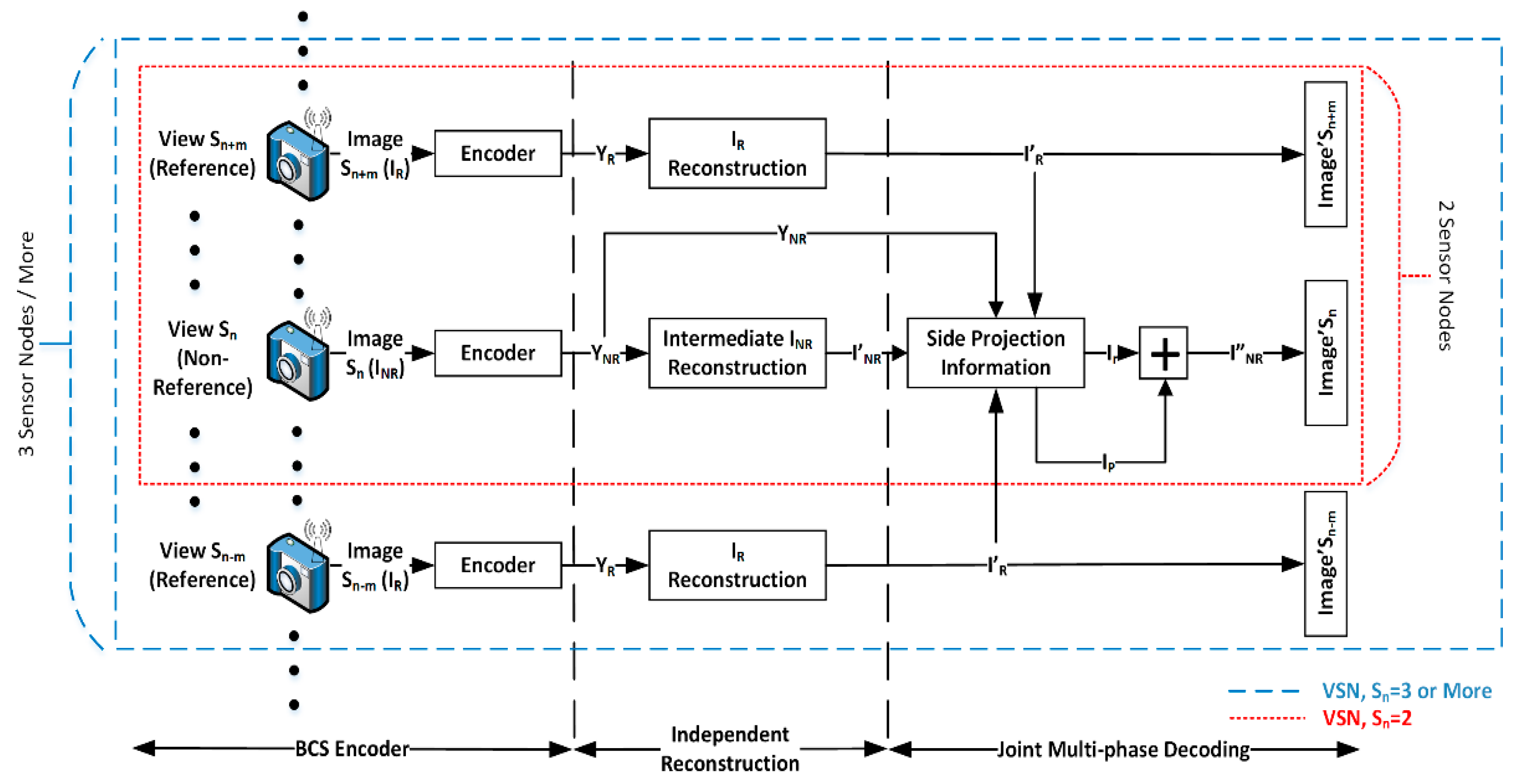
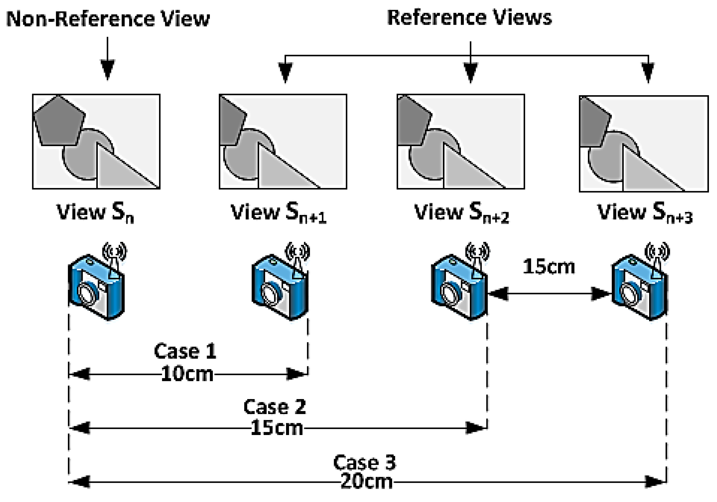
18] is a multi-view compression scheme for VSN based on block-based compressive sensing (BCS) and joint multi-phase decoding (JMD). First, images captured by different visual nodes are encoded using BCS to reduce the hardware complexity. The block-based approach simplifies the implementation and storage of the visual node and provides significantly faster reconstruction. One of the visual nodes is configured to serve as the reference node, whereas the others serve as non-reference nodes. In this case, images captured by the non-reference nodes are encoded at a lower subrate when compared with the images from the reference nodes. The core idea is to improve the reconstruction of images captured by the non-reference nodes, by using information in the image captured by the reference node. It is achieved by exploiting the high correlation between them at the joint-decoder. The encoded measurements are then transmitted independently to the server that serves at the joint-decoder.
At the joint-decoder, the JMD is applied to the received images. The JMD produces and uses side projection information (SPI) to aid the reconstruction of the final image. One reason for using BCS is that it managed to provide an initial reconstruction of an image in a shorter period [
16]. The initial reconstruction helps in the generation of the SPI, which is the core component of the scheme. Besides using the initial reconstruction, residual reconstruction and prediction methods are added to produce an SPI that could better represent the visual data to be decoded. The scheme also works well for both near-field and far-field images, and could also handle parallax and occlusion issues. It is achieved by aligning and fusing the images captured from different view angles. Furthermore, the JMD relies on simplified operations that are less complex when compared to the other reconstruction schemes. Experimental results presented in [
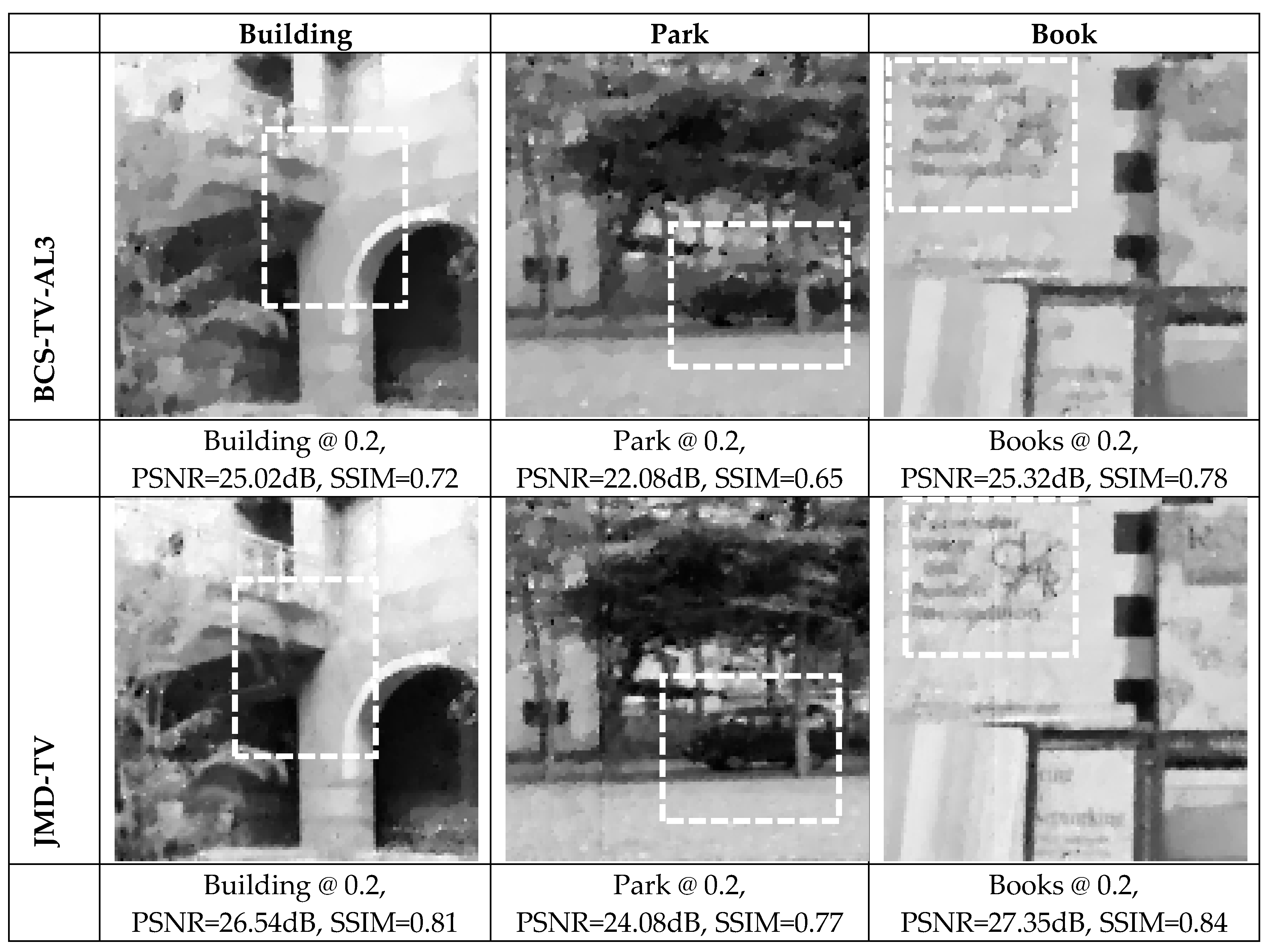
17] show that the BCS-JMD scheme can be applied to images with low, medium, and high texture variations. It can outperform the different independent BCS compressions by a margin of 1.5 dB to 3 dB at various subrates. Furthermore, when compared with other standard multi-view CS compression schemes, the proposed scheme shows a gain of 1.5–2 dB at lower subrates, and the reconstruction speed is also 30–40% shorter. The complete JMD framework is shown in
Figure 9.


