RF Energy Harvesting IoT System for Museum Ambience Control with Deep Learning
Abstract
:1. Introduction and Related Work
1.1. Introduction
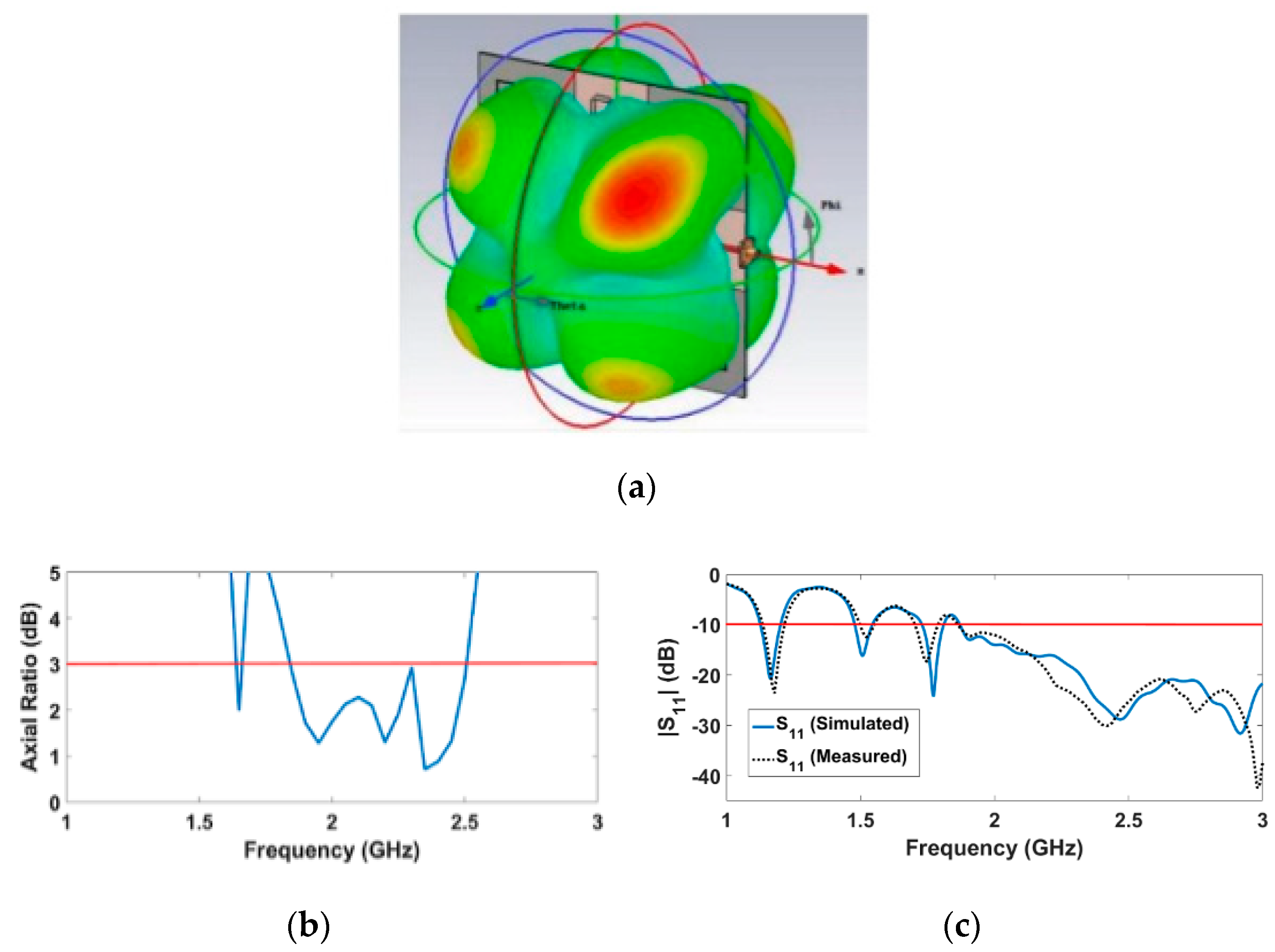
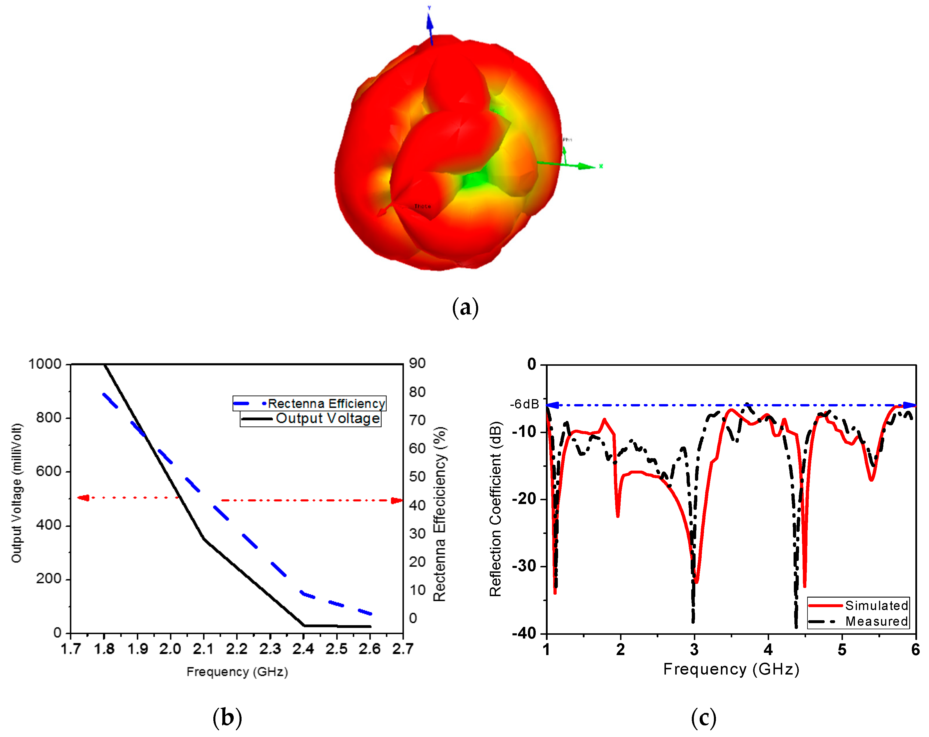
- A complete energy harvesting solution using planar antenna arrays with a simple one-layer structure, integrated with a highly sensitive and simple structure wideband rectifier, which is a suitable solution for powering wireless sensor network an in IoT system. We use two antenna array designs for the RF energy harvesting system to obtain the maximum harvested energy, depending on the scenario in which the system is operating. The first design is a circularly polarized (CP) 2 × 2 antenna array. The second design is a dual linearly polarized antenna array (DLPAA). The complete design of these antennas and some of the other individual elements are presented in [5,6,7,8]. In this paper, we integrate each of the designed antenna arrays with the appropriate rectifier through suitable matching circuits to get maximum power transfer and alleviate the mismatch losses. Furthermore, a power management unit is designed to boost the collected RF energy to charge the battery.
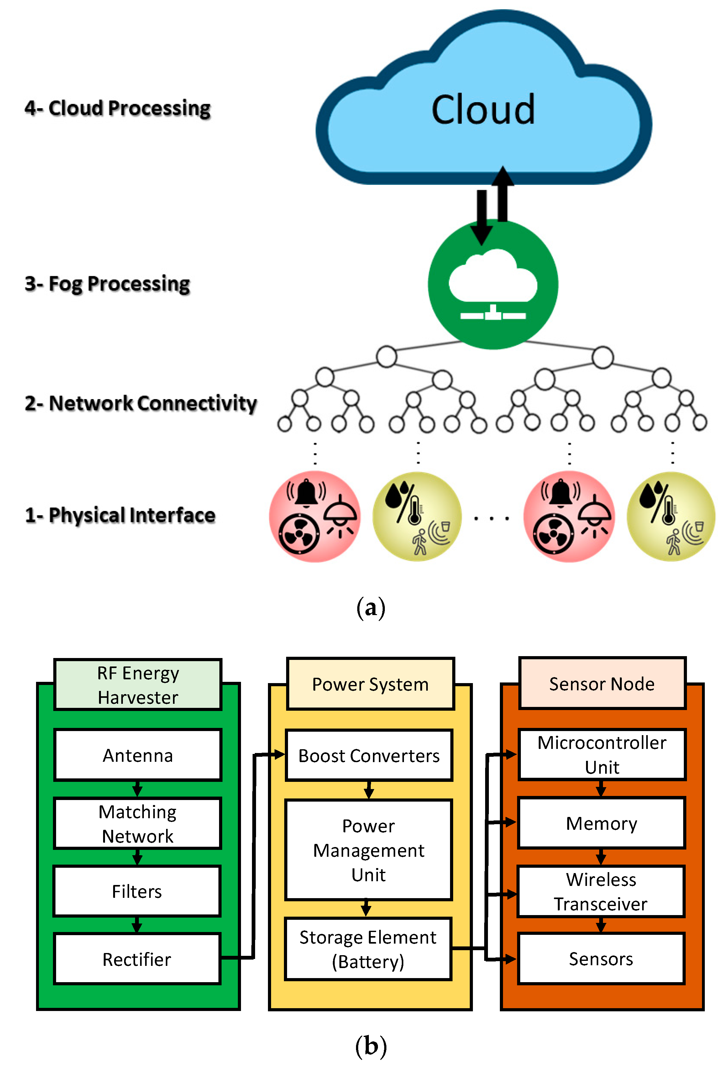
- The development of a layered IoT architecture for museum ambience control based on four layers: (1) A physical interface layer that collects the ambience data and implements decisions developed to control the environment parameters; (2) a network connectivity layer that connects the physical interface layer to the network edge; (3) a fog layer that preprocesses the collected data and performs time-critical actions; and (4) a cloud layer at which the data is stored for further analysis. The building blocks of the architecture are designed for ultra-low-power operation such that it can exploit RF energy harvesting for a prolonged lifetime, despite the use of always-on sensors for occupancy detection and touch detection. This contrasts with existing platforms in the related literature that are battery-powered [2,9,10,11,12], and hence, have a limited lifetime and are incapable of using occupancy and touch-detection sensors.
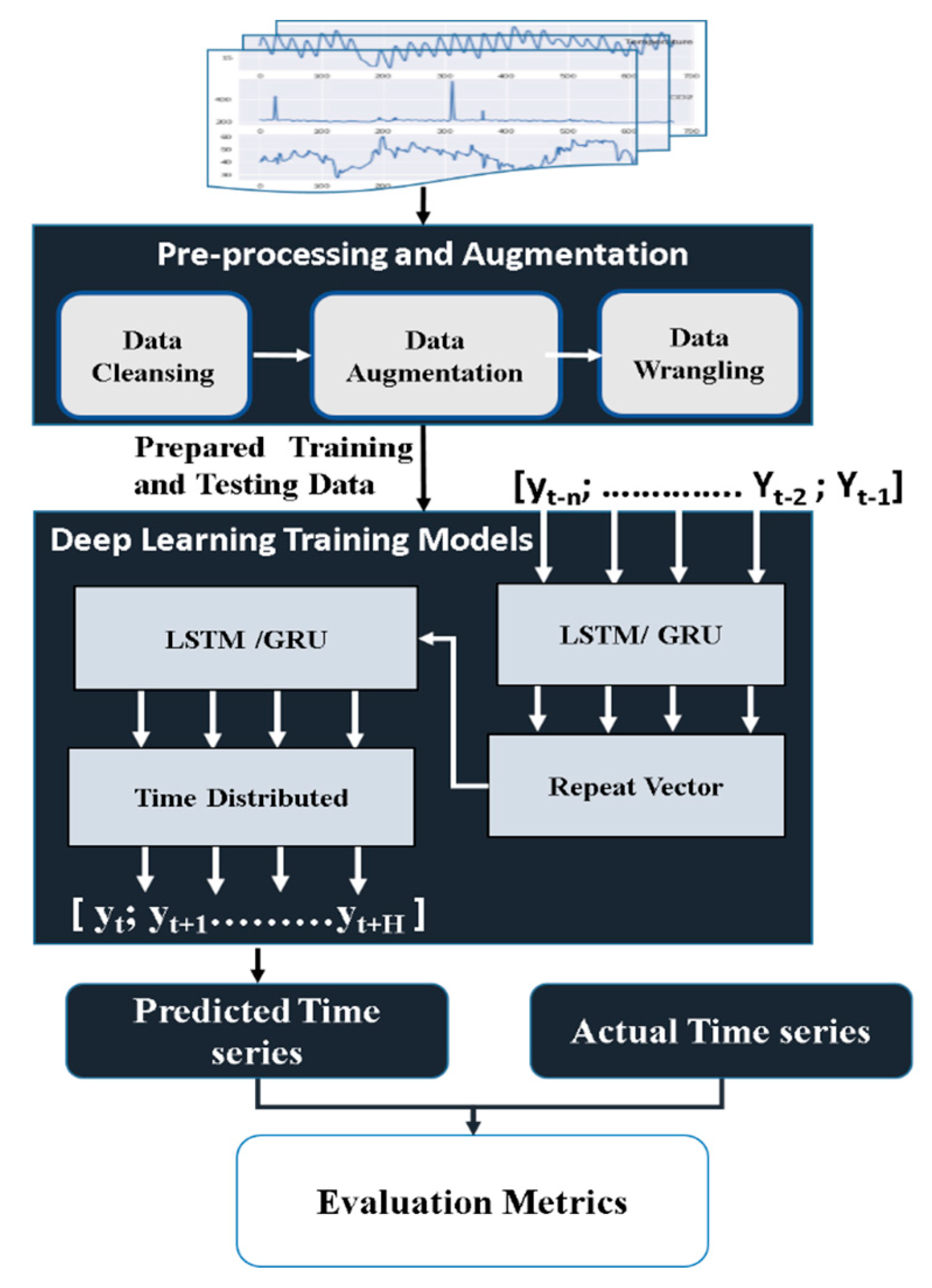
- The development of a deep learning-based framework for indoor air quality prediction and control that predicts the ambience conditions in the upcoming 24 hours. The proposed framework makes the system robust and fault tolerant by providing another source of ambience conditions, such that if the sensors’ readings coming from the IoT system are disrupted for any reason, the museum control is not affected. Furthermore, predicting the future of the ambience helps in creating dynamic ambience control plans with lower energy consumption that provide the basis on which the IoT system operates. This framework enhances our preliminary design presented in [13] by: (1) adding new date-time features (week day, day hour) to consider the effects of working hours and working days, (2) performing correlation analysis to investigate the most suitable predictive variables that affect each other, and (3) using data augmentation to enhance deep learning performance and avoid overfitting. These enhancements significantly reduce errors in predicting environmental attributes by up to 50%, compared to [13].
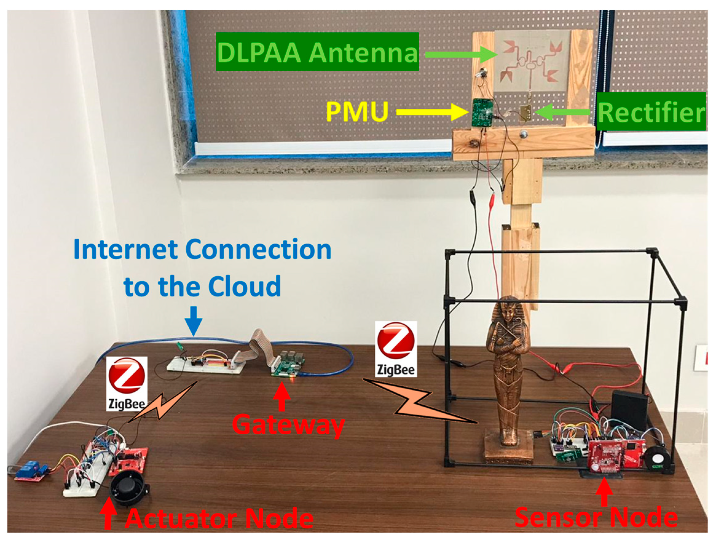
- The implementation of a prototype that integrates the various components of the system. An extensive set of experiments is presented to demonstrate its performance.
1.2. Related Work
1.2.1. Museum Ambience Monitoring and Control
1.2.2. Radio Frequency (RF) Energy Harvesting and Antenna Design
1.2.3. Deep Learning via Time Series Prediction
2. Methodology
2.1. Overall System Description
2.2. RF Energy Harvesting System Design
2.2.1. CP Array Design
2.2.2. DLPAA Design
2.3. Power Management Unit Design
2.4. IoT Architecture and System Design
2.4.1. Physical Interface Layer
2.4.2. Network Connectivity Layer
2.4.3. Fog-Processing Layer
2.4.4. Cloud-Processing Layer
2.5. Deep Learning-based Time Series Prediction
2.5.1. Data Preprocessing and Augmentation
2.5.2. Prediction Phase
3. Results and Discussion
3.1. RF Energy Harvesting Performance
3.2. Power Management Unit Performance
3.3. IoT System Performance
3.4. Time Series Prediction Performance
4. Conclusions
Author Contributions
Funding
Conflicts of Interest
References
- Sharif-Askari, H.; Abu-Hijleh, B. Review of museums’ indoor environment conditions studies and guidelines and their impact on the museums’ artifacts and energy consumption. Build. Environ. 2018, 143, 186–195. [Google Scholar] [CrossRef]
- Shah, J.; Mishra, B. Customized IoT enabled wireless sensing and monitoring platform for preservation of artwork in heritage buildings. In Proceedings of the IEEE International Conference on Wireless Communications, Signal Processing and Networking (WiSPNET), Chennai, India, 23–25 March 2016. [Google Scholar]
- Xie, F.; Yang, G.M.; Geyi, W. Optimal design of an antenna array for energy harvesting. IEEE Antennas Wirel. Propag. Lett. 2013, 12, 155–158. [Google Scholar] [CrossRef]
- Muncuk, U. Design Optimization and Implementation for RF Energy Harvesting Circuits. Master’s Thesis, The Northeastern University, Boston, MA, USA, July 2012. [Google Scholar]
- Elsheakh, D. Broadband dual linear polarized (DLP) antenna array for energy harvesting system. Int. J. Microw. Wirel. Technol. 2019, 1–7. [Google Scholar] [CrossRef]
- Eltresy, N.A.; Elsheakh, D.N.; Abdallah, E.A.; Elhennawy, H.M. Multi-bandwidth CPW-fed open end square loop monopole antenna for energy harvesting. In Proceedings of the 2018 International Applied Computational Electromagnetics Society Symposium (ACES), Denver, CO, USA, 25–29 March 2018. [Google Scholar]
- Dardeer, O.M.; Elsadek, H.A.; Abdallah, E.A. 2 × 2 Circularly Polarized Antenna Array for RF Energy Harvesting in IoT System. In Proceedings of the 2018 IEEE Global Conference on Internet of Things (GCIoT), Alexandria, Egypt, 5–7 December 2018. [Google Scholar]
- Eltresy, N.; Elsheakh, D.; Abdallah, E.; Elhenawy, H. Multi band dual linearly polarized 2 × 2 antenna array for powering sensors in IoT systems. In Proceedings of the IEEE Global Conference on Internet of Things (GCIoT), Alexandria, Egypt, 5–7 December 2018. [Google Scholar]
- Xiao, C.; Chen, N.; Li, D.; Lv, Y.; Gong, J. SCRMS: An RFID and sensor web-enabled smart cultural relics management system. Sensors 2017, 17, 60. [Google Scholar] [CrossRef]
- D’Alvia, L.; Palermo, E.; Rossi, S.; Cappa, P. Development of wireless sensor network for museum environmental monitoring. In Proceedings of the IMEKO International Conference on Metrology for Archeology and Cultural Heritage, Torino, Italy, 19–21 October 2016. [Google Scholar]
- Alsuhly, G.; Khattab, A. An IoT Monitoring and Control Platform for Museum Content Conservation. In Proceedings of the 2018 International Conference on Computer and Applications (ICCA), Beirut, Lebanon, 25–26 July 2018. [Google Scholar]
- De Brito, L.; Peralta, L.; Santos, F.; Fernandes, R. Wireless sensor networks applied to museums’ environmental monitoring. In Proceedings of the 2008 the Fourth International Conference on Wireless and Mobile Communications, Athens, Greece, 27 July–1 August 2008. [Google Scholar]
- Elhariri, E.; Taie, S.A. H-Ahead Multivariate microclimate Forecasting System Based on Deep Learning. In Proceedings of the IEEE International Conference on Innovative Trends in Computer Engineering (ITCE), Aswan, Egypt, 2–4 February 2019. [Google Scholar]
- Kumar, V.D.A.; Saranya, G.; Elangovan, D.; Chiranjeevi, V.R.; Kumar, V.D.A. IoT-Based Smart Museum Using Wearable Device. In International Conference on Innovative Computing and Communications; Springer: Singapore, 2019. [Google Scholar]
- Sornalatha, K.; Kavitha, V.R. IoT based smart museum using Bluetooth Low Energy. In Proceedings of the 2017 Third International Conference on Advances in Electrical, Electronics, Information, Communication and Bio-Informatics (AEEICB), Chennai, India, 27–28 February 2017. [Google Scholar]
- Galletti, A.; Piccialli, F.; Jung, J.E.; De Michele, P.; Cuomo, S. IoT-based collaborative reputation system for associating visitors and artworks in a cultural scenario. Expert Syst. Appl. 2017, 79, 101–111. [Google Scholar]
- Ke, G.; Jiang, Q. Application of Internet of Things technology in the construction of wisdom museum. Concurr. Comput. 2018, 31, e4680. [Google Scholar] [CrossRef]
- Viani, F.; Salucci, M.; Rocca, P.; Oliveri, G.; Massa, A. A multi-sensor WSN backbone for museum monitoring and surveillance. In Proceedings of the 2012 6th European Conference on Antennas and Propagation (EUCAP), Prague, Czech Republic, 26–30 March 2012. [Google Scholar]
- Kim, M.; Suh, T. A low-cost surveillance and information system for museum using visible light communication. IEEE Sens. J. 2019, 19, 1533–1541. [Google Scholar] [CrossRef]
- Sun, H.; Guo, Y.; He, M.; Zhong, Z. A Dual-Band Rectenna Using Broadband Yagi Antenna Array for Ambient RF Power Harvesting. IEEE Antennas Wirel. Propag. Lett. 2013, 12, 918–921. [Google Scholar] [CrossRef]
- Singh, M.; Agrawal, S.; Parihar, M.S. Design of a rectenna system for GSM-900 band using novel broadside 2 × 1 array antenna. J. Eng. 2017, 2017, 232–236. [Google Scholar] [CrossRef]
- Sun, H.; Geyi, W. A New Rectenna Using Beamwidth-Enhanced Antenna Array for RF Power Harvesting Applications. IEEE Antennas Wirel. Propag. Lett. 2017, 16, 1451–1454. [Google Scholar] [CrossRef]
- Guo, Z.; Yang, S.; Shi, Z.; Chen, Y. A miniaturized wideband dual-polarized linear array with balanced antipodal Vivaldi antenna. In Proceedings of the IEEE MTT-S International Microwave Workshop Series on Advanced Materials and Processes for RF and THz Applications (IMWS-AMP), Chengdu, China, 20–22 July 2016. [Google Scholar]
- Haboubi, W.; Takhedmit, H.; Picon, O.; Cirio, L. A GSM-900 MHz and WiFi-2.45 GHz dual-polarized, dual-frequency antenna dedicated to RF energy harvesting applications. In Proceedings of the 2013 7th European Conference on Antennas and Propagation (EuCAP), Gothenburg, Sweden, 8–12 April 2013. [Google Scholar]
- Hamza, H.; Hou, B. Design of trible-band dual-linear polarized microstrip antenna sub-array for SAR applications. In Proceedings of the Asia-Pacific Conference on Antennas and Propagation, Harbin, China, 26–29 July 2014. [Google Scholar]
- Ong, C.S.; Karim, M.; Ong, L.; Chiam, T.; Alphones, A. A compact 2 × 2 circularly polarized antenna array for energy harvesting. In Proceedings of the Asia-Pacific Microwave Conference, Yokohama, Japan, 7–10 December 2010. [Google Scholar]
- Lu, L.; Jiao, Y.C.; Weng, Z.B.; Zhang, L.; Cui, C.Y.; Wang, R.Q. High efficiency circularly-polarized dielectric resonator antenna array fed by the cavity-backed SIW. IEEE Antennas Wirel. Propag. Lett. 2018, 17, 1145–1148. [Google Scholar] [CrossRef]
- Zandikiya, F.; Asadpor, L. Broadband circularly polarized slot antenna array fed by asymmetric CPW for C-band applications. IETE J. Res. 2017, 65, 33–38. [Google Scholar] [CrossRef]
- Handa, R.; Shrivas, A.K.; Hota, H.S. Financial Time Series Forecasting using Back Propagation Neural Network and Deep Learning Architecture. Int. J. Recent Technol. Eng. 2019, 8, 3487–3492. [Google Scholar]
- Aderohunmu, F.A.; Paci, G.; Brunelli, D.; Deng, J.D.; Benini, L.; Purvis, M. An application-specific forecasting algorithm for extending WSN lifetime. In Proceedings of the IEEE International Conference on Distributed Computing in Sensor Systems (DCoSS), Cambridge, MA, USA, 20–23 May 2013. [Google Scholar]
- Milosevic, B.; Caione, C.; Farella, E.; Brunelli, D.; Benini, L. Sub-Sampling framework comparison for Low-Power data gathering: A comparative analysis. Sensors 2015, 15, 5058–5080. [Google Scholar] [CrossRef]
- Wang, W.; Cai, Q.; Wang, S. The research of building indoor temperature prediction based on support vector machine. Adv. Neural Netw. Lect. Notes Comput. Sci. 2014, 8866, 80–89. [Google Scholar]
- Attoue, N.; Shahrour, I.; Younes, R. Smart building: Use of the artificial neural network approach for indoor temperature forecasting. Energies 2018, 11, 395. [Google Scholar] [CrossRef]
- Ahn, J.; Shin, D.; Kim, K.; Yang, J. Indoor air quality analysis using Deep Learning with Sensor Data. Sensors 2017, 17, 2476. [Google Scholar] [CrossRef]
- Tung, N. Multi-band ambient RF energy harvesting rectifier for autonomous Wireless Sensor networks. In Proceedings of the IEEE Region 10 Conference (TENCON), Singapore, 22–25 November 2016. [Google Scholar]
- Barcak, J.M.; Partal, H.P. Efficient RF energy harvesting by using multiband microstrip antenna arrays with multistage rectifiers. In Proceedings of the IEEE Subthreshold Microelectronics Conference (SubVT), Waltham, MA, USA, 9–10 October 2012. [Google Scholar]
- Fu, S.; Fang, S.; Wang, Z.; Li, X. Broadband circularly polarized slot antenna array fed by asymmetric CPW for L-band applications. IEEE Antennas Wirel. Propag. Lett. 2009, 8, 1014–1016. [Google Scholar]
- Manoochehri, O.; Asoodeh, A.; Forooraghi, K. П-Model dual-band impedance transformer for unequal complex impedance loads. IEEE Microw. Wirel. Compon. Lett. 2015, 25, 238–240. [Google Scholar] [CrossRef]
- Skyworks Solutions: SMS7630 Datasheet. Available online: https://datasheet.octopart.com/SMS7630-040LF-Skyworks-Solutions-datasheet-8832283.pdf (accessed on 22 August 2019).
- Texas Instruments. bq25504-Ultra Low Power Boost Converter with Battery Management for Energy Harvester Applications. Tech. Man. 2012. [Google Scholar]
- Yelmarthi, K.; Abdelgawad, A.; Khattab, A. An architectural framework for low-power IoT applications. In Proceedings of the IEEE International Conference on Microelectronics (ICM), Giza, Egypt, 17–20 December 2017. [Google Scholar]
- Texas Instruments: TI-RTOS. Available online: http://processors.wiki.ti.com/index.php/TI-RTOS (accessed on 22 August 2019).
- Zigbee Protocol. Available online: https://en.wikipedia.org/wiki/Zigbee (accessed on 22 August 2019).
- Digi: XBee®/XBee-PRO S2C Zigbee® User Guide. Available online: https://www.digi.com/resources/documentation/digidocs/pdfs/90002002.pdf (accessed on 22 August 2019).
- Node-RED. Available online: https://nodered.org/about/ (accessed on 22 August 2019).
- Forestier, G.; Petitjean, F.; Dau, H.A.; Webb, G.I.; Keogh, E. Generating synthetic time series to augment sparse datasets. In Proceedings of the IEEE International Conference on Data Mining (ICDM), New Orleans, LA, USA, 18–21 November 2017. [Google Scholar]
- Lei, J.; Liu, C.; Jiang, D. Fault diagnosis of wind turbine based on Long Short-Term memory networks. Renew. Energy 2018, 133, 422–432. [Google Scholar] [CrossRef]
- Fu, R.; Zhang, Z.; Li, L. Using LSTM and GRU neural network methods for traffic flow prediction. In Proceedings of the 31st Youth Academic Annual Conference of Chinese Association of Automation (YAC), Wuhan, China, 11–13 November 2016. [Google Scholar]
- Park, S.H.; Kim, B.; Kang, C.M.; Chung, C.C.; Choi, J.W. Sequence-to-sequence prediction of vehicle trajectory via LSTM encoder-decoder architecture. In Proceedings of the IEEE Intelligent Vehicles Symposium (IV), Changshu, China, 26–30 June 2018. [Google Scholar]
- Cho, K.; Van Merriënboer, B.; Gulcehre, C.; Bahdanau, D.; Bougares, F.; Schwenk, H.; Bengio, Y. Learning phrase representations using RNN encoder-decoder for statistical machine translation. In Proceedings of the Empirical Methods in Natural Language Processing (EMNLP), Doha, Qatar, 25–29 October 2014. [Google Scholar]
- Bai, X.; Zhang, J.; Xu, L.J.; Zhao, B. A broadband CPW fractal antenna for RF energy harvesting. In Proceedings of the 2017 International Applied Computational Electromagnetics Society Symposium (ACES), Suzhou, China, 1–4 August 2017; Volume 33, pp. 482–487. [Google Scholar]
- Ladan, S.; Ghassemi, N.; Ghiotto, A.; Wu, K. Highly efficient compact rectenna for wireless energy harvesting application. IEEE Microw. Mag. 2013, 14, 117–122. [Google Scholar] [CrossRef]
- Niotaki, K.; Kim, S.; Jeong, S.; Collado, A.; Georgiadis, A.; Tentzeris, M.M. A compact dual-band rectenna using slot-loaded dual band folded dipole antenna. IEEE Antennas Wirel. Propag. Lett. 2013, 12, 1634–1637. [Google Scholar] [CrossRef]
- Liu, Z.; Zhong, Z.; Guo, Y.X. Enhanced Dual-Band Ambient RF Energy Harvesting with Ultra-Wide Power Range. IEEE Microw. Wirel. Compon. Lett. 2015, 25, 630–632. [Google Scholar] [CrossRef]
- Masotti, D.; Costanzo, A.; Prete, M.D.; Rizzoli, V. Genetic-based design of a tetra-band high-efficiency radio-frequency energy harvesting system. IET Microw. Antenna Prop. 2013, 7, 1254–1263. [Google Scholar] [CrossRef]







| Component’s Part Number | Description |
|---|---|
| CC2650 | Simple link multi-standard ultra-low power wireless microcontroller from Texas Instruments |
| TPL5110 | Nano power system timer |
| HDC1010 | Humidity sensor with a built-in temperature sensor |
| OPT3001 | Ambient light sensor |
| ULPSM-CO 968-001 | Ultra-low power analog sensor module for carbon monoxide |
| GC-0012 | COZIR ultra-low power carbon dioxide sensor |
| LIS3DH | Ultra-low power 3-axis Nano accelerometer |
| BOOSTXL-TLV8544PIR | TLV8544 Quad Nano power Op amp PIR Motion Detector Demonstration Module |
| Freq. (GHz) | V-pol Gain (dBi) | H-pol Gain (dBi) | Rad. Efficiency (%) |
|---|---|---|---|
| 1.8 | 3.5 | 1 | 85 |
| 2.1 | 1.5 | 5.3 | 95 |
| 2.4 | 6.3 | 5.4 | 94 |
| 2.5 | 5.3 | 7.5 | 99 |
| 2.6 | 4.5 | 6.7 | 98 |
| 2.8 | 5.3 | 4 | 99 |
| 2.9 | 3.2 | 1 | 92 |
| Freq. (GHz) | Array Antenna | |
|---|---|---|
| V | H | |
| 1.8 | −34 | −35 |
| 2.1 | −36 | −33 |
| 2.4 | −34 | −33 |
| 2.5 | −35 | −34 |
| 2.6 | −36 | −34 |
| 2.7 | −35 | −36 |
| 2.8 | −36 | −36 |
| 2.9 | −38 | −39 |
| Work | Frequency (GHz) | Antenna Size (mm3) | Maximum Gain (dBi) | Rectenna Efficiency (%) | RF Sensitivity | Load(KΩ) | Polarization Type | Structure Simplicity | Technology |
|---|---|---|---|---|---|---|---|---|---|
| [51] | 0.88–8.45 | 100 × 100 × 1.6 | 8.7 | 51.2% at 2.4 GHz | 0 dBm | 4.7 | Linear | One layer | HSMS-2852 |
| [52] | 0.9 | 62 × 62 × 0.254 | 9 | 60% at 0.9 GHz | 7 dBm | 1 | Linear | One layer | HSMS 2862 |
| [53] | 0.915 and 2.45 | 60 × 60 × 60 | 1.87 and 4.18 | 37% at 0.915 GHz | −9 dBm | 2.2 | Linear | One layer | SMS7630 |
| [54] | 0.915, 1.8 and 2.1 | NA | NA | NA | −15 dBm | 2.1 | NA | NA | HSMS2850 |
| [55] | 0.9, 1.75, 2.15 and 2.45 | 155 × 155 × 1.52 | 9.8 | 59% at 0.9 GHz | -10 dBm | NA | Linear | Two stacked layers | SMS7630 |
| Proposed | 1.8, 2.1, 2.4, and 2.6 | 120 × 130 × 1.525 | 7.5 | 79.5% at 1.8 GHz | −15.5 dBm | 10 | Dual linear polarization and circular polarization | One layer | SMS7630 |
| Architecture | Functionalities | Sensors | Microcontroller | Wireless Transceiver | Current in Sleep | Energy Harvesting | Lifetime Estimate | |
|---|---|---|---|---|---|---|---|---|
| This paper | 4-Layer IoT Architecture | Environmental monitoring & control Occupancy detection Touch detection | T 1, H 2, L 3, CO2, CO, Acc 4, PIR 5 | Texas Instruments CC2650 | XBee Pro X2C | 2.5 mA | Yes | 50.08 days |
| [2] | Adhoc Hopping | Environmental monitoring | T, H, L | PIC24F16KA102 | nRF24L01 | N/A | No | 20 hours |
| [11] | 3-Layer IoT Architecture | Environmental monitoring & control, Occupancy detection, Touch detection | T, H, L, Acc, PIR | Espressif ESP32 | Embedded transceiver | 5.09 mA | No | 9.8 days |
| [12] | Customized | Environmental monitoring | T, H, L, Acc, Bar 6 | MTS400CA | Embedded transceiver | N/A | No | A few days |
| Target Factor | Model | Performance Metric | |||
|---|---|---|---|---|---|
| LSTM | GRU | ||||
| MAE | RMSE | MAE | RMSE | ||
| CO2 | Model 1 | 60.722 | 97.243 | 65.206 | 102.589 |
| Model 2 | 73.353 | 118.201 | 67.252 | 106.115 | |
| Humidity | Model 1 | 2.123 | 2.780 | 1.930 | 2.603 |
| Model 2 | 2.522 | 3.394 | 2.255 | 3.052 | |
| Temperature | Model 1 | 0.683 | 0.847 | 0.722 | 0.911 |
| Model 2 | 0.737 | 0.957 | 0.799 | 1.019 | |
| Indoor Air Quality Factor | Performance Metric | |||
|---|---|---|---|---|
| LSTM | GRU | |||
| MAE | RMSE | MAE | RMSE | |
| CO2 | 63.153 | 94.771 | 59.257 | 101.31 |
| Humidity | 1.893 | 2.708 | 1.861 | 2.630 |
| Temperature | 0.596 | 0.757 | 0.547 | 0.694 |
© 2019 by the authors. Licensee MDPI, Basel, Switzerland. This article is an open access article distributed under the terms and conditions of the Creative Commons Attribution (CC BY) license (http://creativecommons.org/licenses/by/4.0/).
Share and Cite
Eltresy, N.A.; Dardeer, O.M.; Al-Habal, A.; Elhariri, E.; Hassan, A.H.; Khattab, A.; Elsheakh, D.N.; Taie, S.A.; Mostafa, H.; Elsadek, H.A.; et al. RF Energy Harvesting IoT System for Museum Ambience Control with Deep Learning. Sensors 2019, 19, 4465. https://doi.org/10.3390/s19204465
Eltresy NA, Dardeer OM, Al-Habal A, Elhariri E, Hassan AH, Khattab A, Elsheakh DN, Taie SA, Mostafa H, Elsadek HA, et al. RF Energy Harvesting IoT System for Museum Ambience Control with Deep Learning. Sensors. 2019; 19(20):4465. https://doi.org/10.3390/s19204465
Chicago/Turabian StyleEltresy, Nermeen A., Osama M. Dardeer, Awab Al-Habal, Esraa Elhariri, Ali H. Hassan, Ahmed Khattab, Dalia N. Elsheakh, Shereen A. Taie, Hassan Mostafa, Hala A. Elsadek, and et al. 2019. "RF Energy Harvesting IoT System for Museum Ambience Control with Deep Learning" Sensors 19, no. 20: 4465. https://doi.org/10.3390/s19204465
APA StyleEltresy, N. A., Dardeer, O. M., Al-Habal, A., Elhariri, E., Hassan, A. H., Khattab, A., Elsheakh, D. N., Taie, S. A., Mostafa, H., Elsadek, H. A., & Abdallah, E. A. (2019). RF Energy Harvesting IoT System for Museum Ambience Control with Deep Learning. Sensors, 19(20), 4465. https://doi.org/10.3390/s19204465


