1. Introduction
Water provides a material basis for human life and the survival of all living things, and it is an indispensable natural resource needed for the development of human society. Due to population growth, economic development, and changing consumption patterns, the demand for water resources is increasing rapidly, and this increasing demand is expected to accelerate greatly during the next 20 years [
1]. However, the wastage of water resources caused by leakage from water pipelines is an important problem [
2]. A study conducted by the World Bank indicated that the leakage from water pipeline exceeds 48.6 billion
annually, and the corresponding annual economic losses are approximately US
$14.6 billion [
3]. According to the 2012 Green City Index statistics, water pipeline leakage rates exceed 10% in one third of countries worldwide. For example, the average water pipeline leakage rate is 23% in the EU, 13% in the U.S. and Canada, 22% in Asia, 35% in Latin America, and 30% in Africa [
4,
5]. Accordingly, research on high performance water pipeline leakage detection technologies has great significance for the protection of water resources and the promotion of economic development.
The main causes of water pipeline leakage include the corrosive nature of the soil, deficient pipe material quality, the temperature and pressure, failure to employ standard pipe laying methods, geological changes, and human damage [
6,
7,
8]. For instance, deterioration caused by the pressure of the soil may lead to uneven pipeline stress bearing, which can result in leakage from ruptures and breakage. Leakage may also result from damage to pipe junctions caused by external impacts or ruptures caused by the failure to weld junctions during construction. Nevertheless, because the vast majority of water pipelines are located deep underground, leakage is typically not promptly discovered, and when the amount of leakage is large, it is usually not discovered until water begins flowing from the ground surface. Furthermore, since most leaks are relatively small or undetectable, leakage causes substantial waste of water resources [
9,
10]. Therefore, it is extremely important to detect leakage from underground water pipelines effectively and accurately.
Academic researchers and the industry have conducted major research campaigns and developed numerous effective detection methods. One of the earliest detection methods is the listening system in which detection personnel listen to changes in the volume and sound quality of leakage noise coming from equipment and locate areas of leakage based on these observations [
11,
12]. This method not only depends on the experience of the detection personnel, but is highly labor intensive and unreliable due to the large areas of water pipeline networks. Ground penetrating radar can determine the locations of pipeline leaks through the detection of soil voids caused by water leakage. However, because of the complex differences in the geological structure in different areas, this method has poor applicability and is very expensive [
13,
14]. Other studies have presented leakage detection inspired by the changes in the internal pressure of a water pipeline, such as the pressure gradient method, negative pressure wave method, and flow rate balance method [
15,
16,
17]. Although these methods are relatively sensitive to a pipeline’s flow rate and pressure, they tend to give false positive results when the flow rate fluctuations are large because the flow rate in water pipeline networks will fluctuate continuously. It has been found that the spectrum of leakage signals is concentrated, and the pipeline vibration frequency is correlated with the leakage state [
18]. This characteristic can be employed in conjunction with the spectral analysis of signals from piezoelectric accelerometers to perform leakage detection. However, when the environmental noise has a similar frequency spectrum to that of the leakage signals, this method also has a tendency to give false positives. Another study used the linear predictive coding coefficient (LPCC) of acoustic leakage signals and a hidden Markov model (HMM) to improve the ability to distinguish the leakage signal from interfering environmental signals [
19]. However, the detection error of this method tends to increase with the length of time that the system is in use. Furthermore, in [
20,
21,
22], some detection methods based on acoustic signals, such as through hydrophones, have proven that effectively leak detection can be achieved in a longer range of detection in water pipelines. These methods exhibit a high sensitivity to leaks in the range of interest, appearing appropriate for early leak detection. Additionally, the works in [
23,
24,
25] have applied machine learning to pipeline monitoring and have achieved excellent results. Moreover, research on large scale water pipeline network systems has used methods such as real-time modeling to compare measured pipeline network data with flow rate model predictions [
26,
27,
28,
29], but problems such as high modeling difficulty and high computational loads in real applications limit the use of these methods. Researchers have achieved impressive results in research in the field of tap water pipeline leakage detection and location. However, the large scale of water pipeline networks and the extreme complexity of the network architectures, environmental conditions, and geological factors still pose significant challenges for the real-time monitoring of water supply pipeline networks and intelligent leakage detection.
Wireless sensor networks (WSNs) provide an efficient way to address these issues. Due to their outstanding sensing ability, communication protocols, processor speed, and data collection advantages, wireless sensor network technologies have been widely applied in the field of monitoring [
30,
31,
32,
33,
34]. In [
35], PipeNet, a system based on wireless sensor networks, was proposed. It aims to monitor water flow and detect leaks by attaching acoustic and vibration sensors to large bulk-water pipelines and pressure sensors to normal pipelines. In contrast to the PipeNet project, the PipeProbe system does not assume that water pipe surfaces are exposed and accessible for sensor module attachment [
36]. PipeProbe can be dropped into the source of a water pipeline. During its traversal of the pipeline, it collect the sensor readings necessary for the reconstruction of the 3D spatial layout of the traversed water pipelines. To demonstrate the application and control of a low cost wireless sensor network for a high data rate, WaterWiSe@SG, a wireless sensor network to enable real-time monitoring of a water distribution network in Singapore, was proposed in [
37]. The goal of WaterWiSe@SG was to develop generic wireless sensor network capabilities to enable real-time monitoring of a water distribution network.
This paper proposes a water pipeline monitoring system based on wireless sensor networks and a leakage identification method based on support vector machine (SVM). Machine learning can simulate the acquisition of knowledge through human learning activities and can enable the automatic improvement of system performance. As a result, it is widely applied in speech and biological affect identification [
38], physiological signal detection [
39], body movement identification [
40], signal feature detection and identification, etc. [
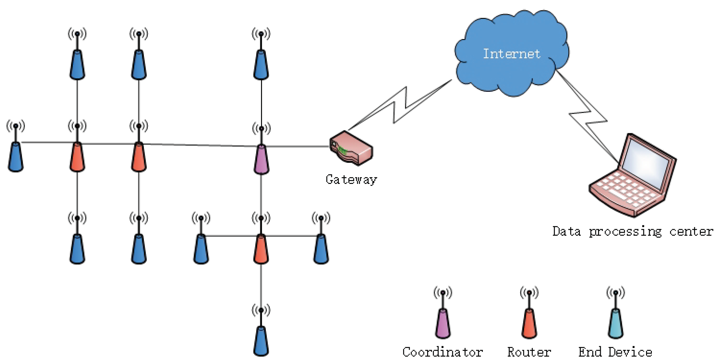
41,
42,
43,
44]. The proposed system employs ZigBee nodes serving as signal collection nodes and uses the 4G network to transmit the signals adopted by the sensors to the data processing center for processing. To address the high networking power consumption that affects conventional wireless sensor networks, we also propose a leakage triggered networking method able to network and perform data transmission from wireless sensor nodes in the vicinity of leakage points, which effectively reduces the network energy consumption and extends its life cycle. Based on the differences in the time-frequency features of leakage and non-leakage signals, we propose a leakage detection method that constructs feature matrices by employing the intrinsic mode function, approximate entropy, and principal component analysis (PCA) and that uses SVM as a classifier to identify the leaks. Our experiment is performed along an exposed aluminum-plastic composite pipe, with a diameter of 27 mm. The CT1010 acceleration sensor is used in this experiment due to its sensitivity. During our experiments, the water pressure is no less than 0.3 MPa. The detectable leaking flow rate is calculated to be approximately 2.5 cm
/s based on the pipe pressure. Experimental and simulation results demonstrate that the proposed methods can effectively detect the leakage and prolong the lifetime of the wireless sensor network.
The rest of the paper is organized as follows. The implementation of the leakage monitoring system is introduced in
Section 2. In
Section 3, the leakage triggered networking solution for wireless sensor networks that are able to network sensors receiving leakage signals is developed. We propose a leakage detection method based on time-frequency features and SVM in
Section 4. Experimental and simulations results are reported in
Section 5. Conclusions are presented in
Section 6.
3. Leakage Triggered ZigBee Networking
In actual water pipeline monitoring environments, a large number of terminal sensors needs to be installed along pipelines. Since the pipeline leakage is a low probability event, all of the sensors working at the same time will result in a significant waste of energy. Furthermore, leakage in water supply pipelines occurs randomly, and pipeline systems must be monitored in real time. To reduce energy consumption and increase network lifetime, we propose a leakage triggered networking method.
The ZigBee networking method includes initialization networking and triggered networking. The topological structure of the network provides an important basis for ZigBee networking; in view of the structural characteristics and distribution of water supply pipelines, this paper employed a network topology. To achieve initialization networking, the first step was to determine the coordinator nodes and set their signal channels and network ID numbers, which would initialize the network. Non-coordinator nodes were then added to the network.
Figure 3 mainly interprets how the nodes join the network. To ensure that the number of terminal nodes installed at each relay node (i.e., router node) was balanced, it would add received signal strength indicator (RSSI) information to each Beacon_request frame when each terminal node in this solution sends a network join request. In accordance with the RSSI values, routing nodes provided joining service to the terminal nodes. To collect leakage signals effectively and reliably, it is necessary to set reasonable threshold values for the RSSI. If the RSSI values of the terminal nodes are smaller than the threshold, the routing nodes will not process the request of terminal nodes. If the RSSI values are greater than the threshold, the routing nodes will record the terminal nodes’ information and ensure that they can join the network.
After the network was initialized, to reduce the network power consumption and prolong the network lifetime, this paper designed three types of control frames (i.e., join frame, active frame, and wave frame), which can be used to trigger the network according to the leakage detection results. The structures of the join frame, active frame, and wave frame are shown in
Table 1,
Table 2 and
Table 3. The Sou_address field is the original address, which is the routing node address. The nodes rely on this field to determine whether they have been activated and are working. The Des_address field is the destination address and constitutes the address of a routing node that has joined the network. The PANID is the network address. In the join frames, the join_result field is the result of networking; a result of zero indicates that the networking of a routing node has failed, and a result of one indicates that it has been successful. In the active frame, the Act_address field is the active address, and child nodes will join the network after receiving this information and then perform data sampling. In the wave frames, the Position field records the actual physical address information. Because this paper mainly considered the networking solution and its performance, the Position field was not used for node location.
Figure 4 shows the leakage triggered networking flowchart. The terminal nodes send Join frames to the routing nodes to compile a list of terminal nodes. After the routing-terminal relationship has been constructed, the routing nodes will send Active frames to the terminal nodes. When receiving Active frames, the terminal nodes will then determine whether they are the destination nodes. If a node is a destination node, it will activate itself and perform data sampling. If a node is not a destination node, it will enter a sleep monitoring state and wait for the next Active frame. Once a node in the working state determines that a signal it has received is a leakage signal, the routing node will send the preset leakage triggered address to the nodes on the terminal nodes list. All of the nodes on the list receiving that address will activate themselves and initiate signal sampling and transmission. This method enables routing nodes to control the working status of the terminal nodes. After the networking is completed, data transmission is performed using the ZigBee routing protocol.
5. Simulation Results
5.1. Leakage Triggered Networking
In this section, OPNET Modeler14.5 was used to simulate the proposed leakage triggered networking method. The simulation process requires the design and configuration of three different layers. The node layer defines the node behavior and controls the data flow between the different modules in one node. The process layer uses the protocol to perform state conversion for the state machines. The network layer establishes the network topological structure and network layers.
Generally, a ZigBee node model includes an application layer, network layer, MAC layer, and a wireless transceiver. To compile the network power consumption, we added an energy calculation module to the node model. The energy calculation module kept track of the transceiver’s standby, receiving, and transmitting energy consumption via monitoring of the transceiver status. Since the code for the application layer module and network layer module in OPNET was not available, we redesigned the application layer and network layer modules. During the simulation, the coordinator nodes, routing nodes, and terminal nodes had the same node model. The application layer included the source module and sink module. The source module employed the simple_source model, which was a data packet generation module and was responsible for generating data packets with the specified packet size in accordance with the specified packet interval. The sink module was a data packet destruction module and was responsible for destroying data packets that had been transmitted to the destination node, which released internal storage dynamically assigned by the program. The network layer consisted of the network_layer module and mainly served to drive the completion of networking procedures by the MAC module, complete initialization networking and leakage triggered networking, and perform data packet routing in accordance with the AODVjrrouting protocol. The MAC layer employed an 802_15_4_mac module and had a CSMA/CA competitive algorithm. The 802_15_4_mac module performed some networking, multiple access, and sleep management functions via an added sleep state machine. The physical layer employed a wireless_tx/wireless_rx module as a wireless transceiver.
The water supply pipeline network shown in
Figure 9 was designed for the simulation. The area was 1500 m × 1500 m and contained a total of 644 ZigBee nodes, which included six coordinator nodes and 638 routing and terminal nodes. The coordinator nodes were considered as sink nodes. The distance between adjacent nodes was 10 m; the distance between routing nodes was 50 m; and four terminal nodes were located between each pair of routing nodes. Each of the routing and terminal nodes was also a sensor. The terminal nodes completed the data collection and the detection of the water leakage signal and sent the data to the routing nodes. Then, the routing nodes transmitted the information collected by themselves and the terminal nodes to the sink nodes through multi-hop routing. Finally, the sink nodes sent the information to the background control center to realize the monitoring of the entire network. An RxGroup Configmo module was used to configure the nodes’ single-hop link distance in the simulation scenario, and channel fading employed a free space loss model. The simulation parameters for each layer are shown in
Table 4.
The simulation time was 1200 s. First, leakage signal information functions were established in the MAC layer, and a leakage triggered networking experiment was performed via the establishment of leakage point coordinates, signal attenuation coefficients, and the leakage signal detection threshold using the functions. The leakage coordinate was (319, 753), which indicated that the leakage point was located between Nodes 10 and 11, as shown in
Figure 10. In the simulation, Node 3 was a coordinator node, Nodes 8, 13, and 18 were routing nodes, and the remaining nodes were terminal nodes. According to the simulation settings, leakage occurred at 700–720 s, and the signal attenuation coefficient and leakage signal detection threshold settings ensured that Routing Nodes 8 and 13 could receive the leakage signal. We also monitored the active and sleep status of the MAC layer to track the nodes’ networking status.
Figure 11 shows the working statuses during the 0–1200 s period. The coordinator and routing nodes were consistently in the working state, and the terminal nodes within the routing node network were sequentially working and sleeping. Leakage occurred when the simulation time reached 700 s, and all of the terminal nodes within the network formed by Routing Nodes 8 and 13 entered the working state at that time. Leakage ceased when the simulation time reached 720 s, and the terminal nodes within the network formed by Routing Nodes 8 and 13 resumed the normal working status. The routing nodes on both sides of the leakage point could detect the leakage signal and performed networking when the leakage occurred, whereas the other routing nodes remained in a normal working state. Simulation results indicated that the proposed solution achieved leakage triggered networking by the sensor nodes on both sides of a leakage point, which could further provide data to determine the location of the leakage point.
Figure 12 shows a comparison of the networking time between the proposed networking solution and the ZigBee 2007 networking solution. The simulation results indicated that the networking time of the proposed solution was slightly greater than that of the ZigBee 2007 solution because of the addition of the RSSI threshold value. However, the networking time of all the nodes increased only by approximately 1.39%. Therefore, the proposed solution could be used in a large scale networking environment.
Figure 13 shows a comparison of the power and energy consumptions of the proposed solution and the ZigBee 2007 solution. Simulation results clearly demonstrated that the proposed solution could reduce the network power and energy consumption and increase the network lifetime through controlling of the polling work of the terminal nodes within their networks.
Figure 14 shows the percentage of terminal nodes carried by all the routing nodes when the transmission power of the sensor nodes was 1 mW and the RSSI threshold was −68 dBm. In accordance with the channel loss model, the signal transmission distance controlled by the threshold value was approximately 25 m. Because the nodes were spaced at intervals of 10 m in the simulation, four terminal nodes were carried by each routing node. The results shown in
Figure 14 indicate that the proposed solution can ensure the number of terminal nodes carried by the routing nodes was more uniform than that in the original solution and could thereby ensure more stable network coverage.
5.2. Leakage Identification
The experiment was performed along an exposed aluminum-plastic composite pipe, with a diameter of 27 mm. Moreover, the water-tap was used as the leakage sound source, then the flow rate was adjusted, and the sensor was placed at a distance of 20 cm away from the water-tap. One hundred datasets of leakage signals and non-leakage signals were sampled respectively. Each dataset had a length of 5000, and the data were used to train and optimize the SVM model. In addition, 100 datasets of leakage and non-leakage signals were sampled during the early quiet morning hours, respectively. Therefore, the simulated noise was employed to verify the effectiveness of the proposed leakage detection.
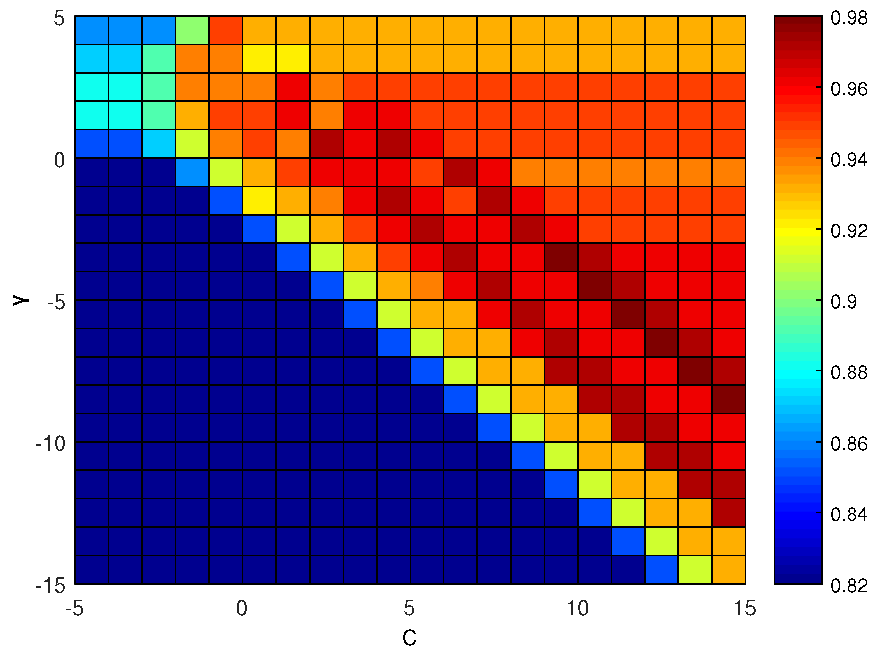
At first, 50 datasets were extracted from each of the leakage and non-leakage signals and used to create a training set. The remaining samples were then used to create a testing set. The SVM parameters
were set to an integer power of two; the range of
C was set as
; and the range of
was set as
. The grid-search method was used, and
for
parameter combinations were used to perform the model training. The detection accuracy is shown in
Figure 15. The results indicated that the highest identification accuracy achieved by the proposed algorithm was 98%. In addition, when
,
, and
, the SVM model based on the radial basis kernel provided good pipeline leakage signal identification performance.
To verify the effectiveness of the proposed leakage detection, the experiment was performed in which 100 datasets of leakage signals and non-leakage signals were sampled, respectively.
Figure 16 shows the detection results for
parameter combinations, where the leakage label was 2, and the non-leakage label was 1. The identification results showed that the proposed method only determined two leakage signals to be non-leakage signals and made accurate determinations in all other cases, indicating that the classification accuracy achieved by the proposed algorithm was 98%.
Table 5 shows the results obtained by using the proposed algorithm to perform leakage identification after artificial Gaussian noise and impulsive noise were added to leakage signals obtained during a quiet period of time. The results indicated that the proposed water supply pipeline leakage detection method based on the time-frequency features of the signal and SVM could effectively detect pipeline leakage.


