Strip Adjustment of Airborne LiDAR Data in Urban Scenes Using Planar Features by the Minimum Hausdorff Distance


Abstract
:1. Introduction
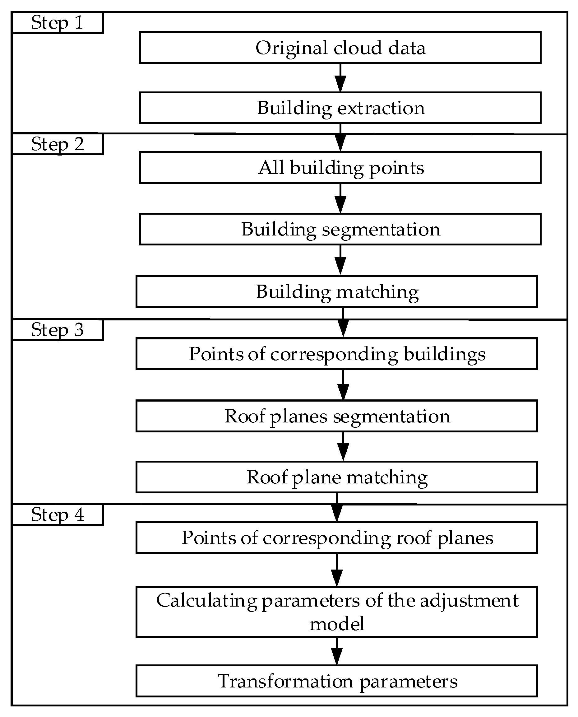
2. Methodology
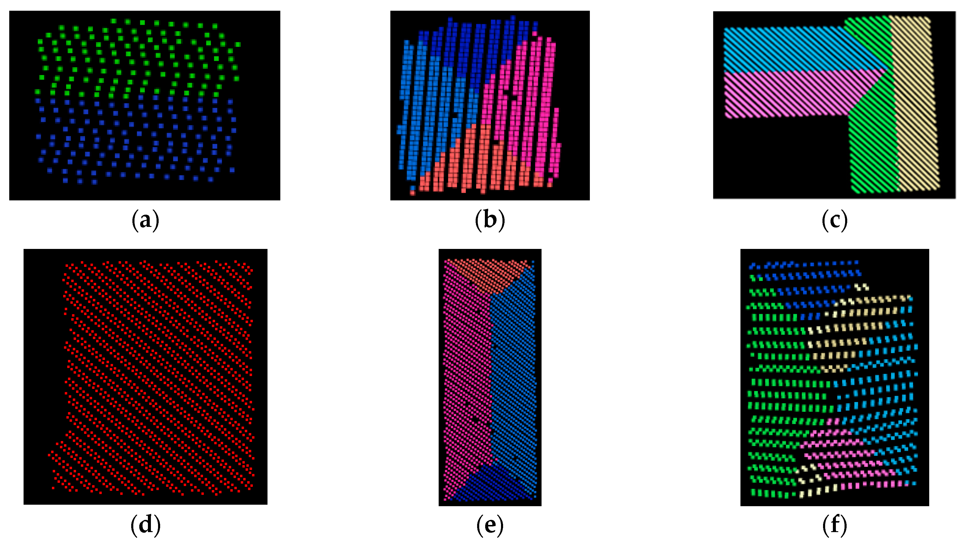
2.1. Building Segmentation
2.2. Building Matching
2.3. Roof Plane Segmentation
2.3.1. Preprocessing the Point Cloud of Buildings
2.3.2. Coarse-to-Fine Segmentation Algorithm
2.4. Roof Plane Matching
2.5. Mathematical Model for Adjustment Computation
3. Results
3.1. Experiment of Single Channel LiDAR Data
3.1.1. Data Description
3.1.2. Results of Building Matching and Planar Patch Segmentation
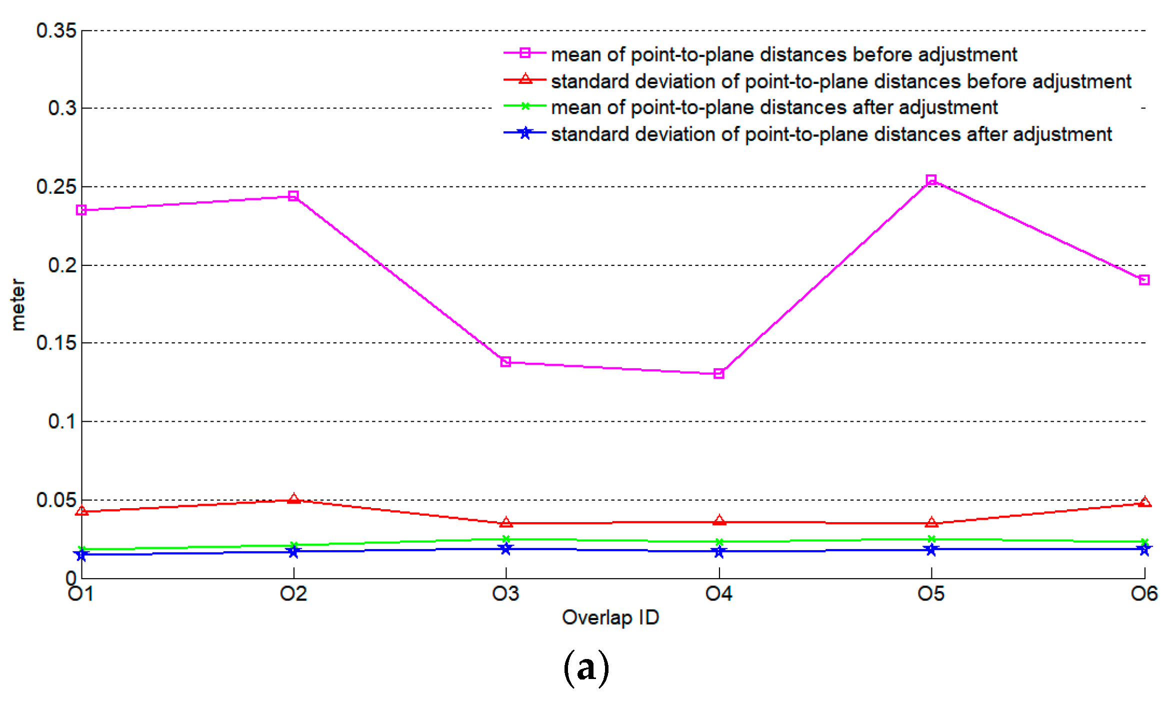
3.1.3. Parameters Estimation and Evaluation
3.2. Experiment of Dual Channel LiDAR Data
3.2.1. System and Data Description
3.2.2. Results of Building Matching and Planar Patch Segmentation
3.2.3. Final Results
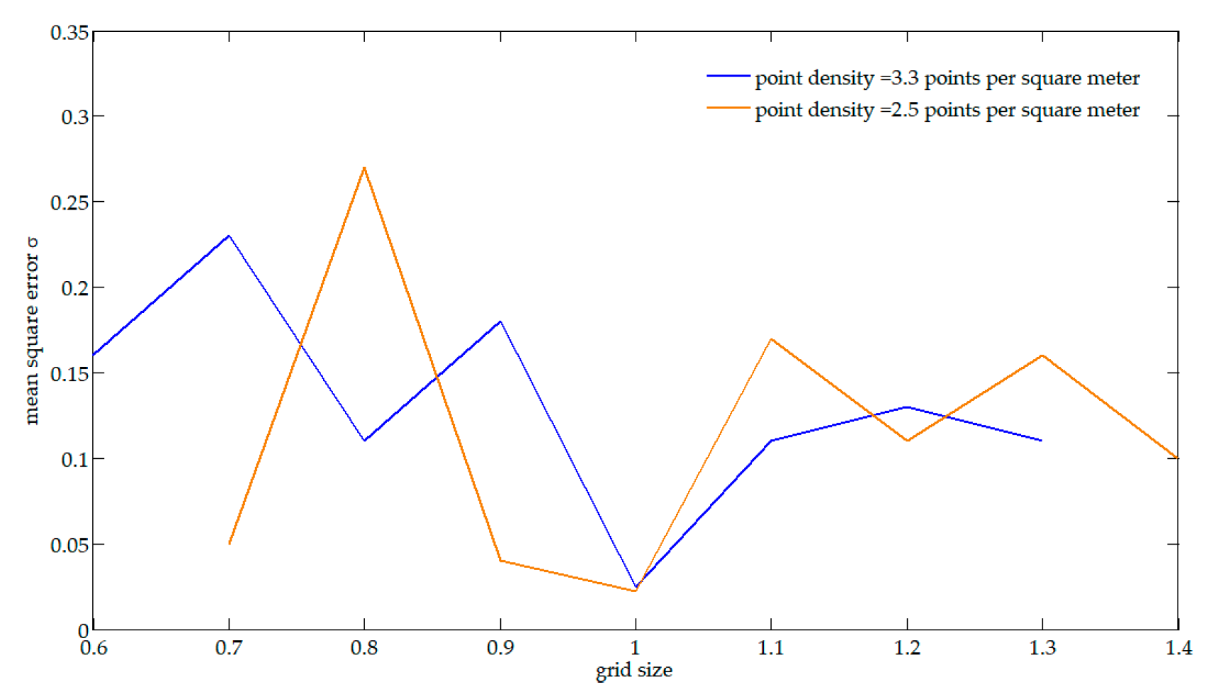
3.3. Discussion on the Pixel Size of the Binary Image
3.4. Discussion on the Order of Strip Pairs for Adjustment
4. Discussion
Author Contributions
Funding
Conflicts of Interest
References
- Yi, C.; Zhang, Y.; Wu, Q.; Xu, Y.; Remil, O.; Wei, M.; Wang, J. Urban building reconstruction from raw LiDAR point data. Comput. Aided Des. 2017, 93, 1–14. [Google Scholar] [CrossRef]
- Hui, Z.; Hu, Y.; Jin, S.; Yevenyo, Y. Road centerline extraction from airborne LiDAR Point cloud based on hierarchical fusion and optimization. ISPRS J. Photogramm. Remote Sens. 2016, 118, 22–36. [Google Scholar] [CrossRef]
- Zhao, Z.; Duan, Y.; Zhang, Y.; Cao, R. Extracting buildings from and regularizing boundaries in airborne lidar data using connected operators. Int. J. Remote Sens. 2016, 37, 889–912. [Google Scholar] [CrossRef]
- Tran, T.; Ressl, C.; Pfeifer, N. Integrated change detection and classification in urban area based on airborne laser scanning point clouds. Sensors 2018, 18, 448. [Google Scholar] [CrossRef] [PubMed]
- Dong, P.; Ramesh, S.; Nepali, A. Evaluation of small-area population estimation using LiDAR, Landsat TM and parcel data. Int. J. Remote Sens. 2010, 31, 5571–5586. [Google Scholar] [CrossRef]
- Stal, C.; Tack, F.; de Maeyer, P.; de Wulf, A.; Goossens, R. Airborne photogrammetry and lidar for DSM extraction and 3D change detection over an urban area—A comparative study. Int. J. Remote Sens. 2013, 34, 1087–1110. [Google Scholar] [CrossRef]
- Polat, N.; Uysal, M. Investigating performance of airborne LiDAR data filtering algorithms for DTM generation. Measurement 2015, 63, 61–68. [Google Scholar] [CrossRef]
- Jo, J.H.; Rose, Z.; Cross, J.; Daebel, E.; Verderber, A.; Kostelnick, J.C. Application of airborne LiDAR data and geographic information systems (GIS) to develop a distributed generation system for the town of normal, IL. AIMS Energy 2015, 3, 173–183. [Google Scholar] [CrossRef]
- Skaloud, J.; Lichti, D. Rigorous approach to bore-sight self-calibration in airborne laser scanning. ISPRS J. Photogramm. Remote Sens. 2006, 61, 47–59. [Google Scholar] [CrossRef]
- Huising, E.J.; Pereira, L.M. Errors and accuracy estimates of laser data acquired by various laser scanning systems for topographic applications. ISPRS J. Photogramm. Remote Sens. 1998, 53, 245–261. [Google Scholar] [CrossRef]
- Bang, K.I.; Habib, A.; Kersting, A. Estimation of biases in lidar system calibration parameters using overlapping strips. Can. J. Remote Sens. 2010, 36, S335–S354. [Google Scholar] [CrossRef]
- Hodgson, M.E.; Bresnahan, P. Accuracy of airborne lidar-derived elevation. Photogramm. Eng. Remote Sens. 2004, 70, 331–339. [Google Scholar] [CrossRef]
- Zhang, Y.; Xiong, X.; Zheng, M.; Xu, H. LiDAR strip adjustment using multifeatures matched with aerial images. IEEE Trans. Geosci. Remote Sens. 2015, 53, 976–987. [Google Scholar] [CrossRef]
- Rottensteiner, F.; Weser, T.; Lewis, A.; Fraser, C.S. A strip adjustment approach for precise georeferencing of ALOS optical imagery. IEEE Trans. Geosci. Remote Sens. 2009, 47, 4083–4091. [Google Scholar] [CrossRef]
- Kilian, J.; Haala, N.; Englich, M. Capture and evaluation of airborne laser scanner data. Int. Arch. Photogramm. Remote Sens. 1996, 31, 383–388. [Google Scholar]
- Crombaghs, M.; Brügelmann, R.; de Min, E.J. On the adjustment of overlapping strips of laser altimeter height data. Int. Arch. Photogramm. Remote Sens. 2000, 33, 230–237. [Google Scholar]
- Wu, H.; Fan, H. Registration of airborne LiDAR point clouds by matching the linear plane features of building roof facets. Remote Sens. 2016, 8, 447. [Google Scholar] [CrossRef]
- Habib, A.F.; Kersting, A.P.; Bang, K.I.; Zhai, R.; AI-Durgham, M. A strip adjustment procedure to mitigate the impact of inaccurate mounting parameters in parallel LiDAR strips. Photogramm. Rec. 2009, 24, 171–195. [Google Scholar] [CrossRef]
- Sande, C.V.; Soudarissanane, S.; Khoshelham, K. Assessment of relative accuracy of AHN-2 laser scanning data using planar features. Sensors 2010, 10, 8198–8214. [Google Scholar] [CrossRef]
- Pfeifer, N.; Elberink, S.O.; Filin, S. Automatic tie elements detection for laser scanner strip adjustment. Int. Arch. Photogramm. Remote Sens. 2005, 36, 1682–1750. [Google Scholar]
- Filin, S. Analysis and implementation of a laser strip adjustment model. Int. Arch. Photogramm. Remote Sens. 2003, 34, 65–70. [Google Scholar]
- Lee, J.; Yu, K.; Kim, Y.; Habib, A.F. Adjustment of discrepancies between LiDAR data strips using linear features. IEEE Geosci. Remote Sens. Lett. 2007, 4, 475–479. [Google Scholar] [CrossRef]
- Habib, A.F.; Kersting, A.P.; Ruifang, Z.; Durgham, M.; Kim, C.; Lee, D.C. LiDAR strip adjustment using conjugate linear features in overlapping strips. In Proceedings of the International Archives of the Photogrammetry, Remote Sensing and Spatial Information Sciences, Beijing, China, 3–11 July 2008; pp. 385–390. [Google Scholar]
- Rentsch, M.; Krzystek, P. LiDAR strip adjustment using automatically reconstructed roof shapes. In Proceedings of the International Archives of the Photogrammetry, Remote Sensing and Spatial Information Science, Hannover, Germany, 2–5 June 2009; pp. 158–164. [Google Scholar]
- Terrasolid. Available online: http://www.terrasolid.com/home.php (accessed on 26 October 2019).
- Axelsson, P. Processing of laser scanner data-algorithms and applications. ISPRS J. Photogramm. Remote Sens. 1999, 54, 138–147. [Google Scholar] [CrossRef]
- Ma, H.; Zhou, W.; Zhang, L. DEM refinement by low vegetation removal based on the combination of full waveform data and progressive TIN densification. ISPRS J. Photogramm. Remote Sens. 2018, 146, 260–271. [Google Scholar] [CrossRef]
- Cai, Z.; Ma, H.; Zhang, L. A Building detection method based on semi-suppressed fuzzy C-means and restricted region growing using airborne LiDAR. Remote Sens. 2019, 11, 1–18. [Google Scholar] [CrossRef]
- Rodríguez-Caballero, E.; Afana, A.; Chamizo, S.; Solé-Benet, A.; Canton, Y. A new adaptive method to filter terrestrial laser scanner point clouds using morphological filters and spectral information to conserve surface micro-topography. ISPRS J. Photogramm. Remote Sens. 2016, 117, 141–148. [Google Scholar] [CrossRef]
- Ge, X. Automatic markerless registration of point clouds with semantic-keypoint-based 4-points congruent sets. ISPRS J. Photogramm. Remote Sens. 2017, 130, 344–357. [Google Scholar] [CrossRef]
- Lin, Y.; Wang, C.; Cheng, J.; Chen, B.; Jia, F.; Chen, Z.; Li, J. Line segment extraction for large scale unorganized point clouds. ISPRS J. Photogramm. Remote Sens. 2015, 102, 172–183. [Google Scholar] [CrossRef]
- Hui, Z.; Hu, Y.; Yevenyo, Y.; Yu, X. An improved morphological algorithm for filtering airborne LiDAR point cloud based on multi-level kriging interpolation. Remote Sens. 2016, 8, 35. [Google Scholar] [CrossRef]
- He, L.; Ren, X.; Gao, Q.; Zhao, X.; Yao, B.; Chao, Y. The connected-component labeling problem: A review of state-of-the-art algorithms. Pattern Recognit. 2017, 70, 25–43. [Google Scholar] [CrossRef]
- Haralick, R.; Shapiro, L. Computer and Robot Vision, 1st ed.; Addison-Wesley: Reading, MA, USA, 1992; pp. 28–32. [Google Scholar] [CrossRef]
- Di Stefano, L.; Bulgarelli, A. A simple and efficient connected components labeling algorithm. In Proceedings of the 10th International Conference on Image Analysis and Processing, Los Alamitos, CA, USA, 27–29 September 1999; pp. 322–327. [Google Scholar] [CrossRef]
- Baudrier, E.; Millon, G.; Nicolier, F.; Seulin, R.; Ruan, S. Hausdorff distance-based multiresolution maps applied to image similarity measure. Imaging Sci. J. 2007, 55, 164–174. [Google Scholar] [CrossRef]
- He, B.; Lin, Z.; Li, Y.F. An automatic registration algorithm for the scattered point clouds based on the curvature feature. Opt. Laser Technol. 2013, 46, 53–60. [Google Scholar] [CrossRef]
- Fischer, A.; Suen, C.Y.; Frinken, V.; Riesen, K.; Bunke, H. Approximation of graph edit distance based on Hausdorff matching. Pattern Recognit. 2015, 48, 331–343. [Google Scholar] [CrossRef]
- Huttenlocher, D.P.; Klanderman, G.A.; Rucklidge, W.J. Comparing images using the Hausdorff distance. IEEE Trans. Pattern Anal. Mach. Intell. 1993, 15, 850–863. [Google Scholar] [CrossRef]
- Chen, Y.; He, F.; Wu, Y.; Hou, N. A local start search algorithm to compute exact Hausdorff Distance for arbitrary point sets. Pattern Recognit. 2017, 67, 139–148. [Google Scholar] [CrossRef]
- Taha, A.A.; Hanbury, A. An efficient algorithm for calculating the exact Hausdorff distance. IEEE Trans. Pattern Anal. Mach Intell. 2015, 37, 2153–2163. [Google Scholar] [CrossRef]
- Zhang, D.; He, F.; Han, S.; Zou, L.; Wu, Y.; Chen, Y. An efficient approach to directly compute the exact Hausdorff distance for 3D point sets. Integr. Comput. Aided Eng. 2017, 24, 261–277. [Google Scholar] [CrossRef] [Green Version]
- Zhao, R.; Pang, M.; Wei, M. Accurate extraction of building roofs from airborne light detection and ranging point clouds using a coarse-to-fine approach. J. Appl. Remote Sens. 2018, 12, 1–14. [Google Scholar] [CrossRef]
- Kornus, W.; Ruiz, A. Strip adjustment of LiDAR data. Int. Arch. Photogramm. Remote Sens. 2003, 34, 47–50. [Google Scholar]
- Maas, H.G. Methods for measuring height and planimetry discrepancies in airborne laserscanner data. Photogramm. Eng. Remote Sens. 2002, 68, 933–940. [Google Scholar]
- Bosché, F. Plane-based registration of construction laser scans with 3D/4D building models. Adv. Eng. Inform. 2012, 26, 90–102. [Google Scholar] [CrossRef]
- Filin, S. Recovery of systematic biases in laser altimetry data using natural surfaces. Photogramm. Eng. Remote Sens. 2003, 69, 1235–1242. [Google Scholar] [CrossRef]
- Burman, H. Laser strip adjustment for data calibration and verification. Int. Arch. Photogramm. Remote Sens. 2002, 34, 67–72. [Google Scholar]
- Lee, J.; Han, D.; Yu, K.; Heo, J.; Habib, A. An automatic registration method for adjustment of relative elevation discrepancies between lidar data strips. GIsci. Remote Sens. 2010, 47, 115–134. [Google Scholar] [CrossRef]
- Zhang, X.; Zang, A.; Agam, G.; Chen, X. Learning from synthetic models for roof style classification in point clouds. In Proceedings of the 22nd ACM SIGSPATIAL International Conference on Advances in Geographic Information Systems, Dallas, TX, USA, 4–7 November 2014; pp. 263–270. [Google Scholar] [CrossRef]
- Van Rees, E. Trimble’s AX60i and AX80. GeoInformatics 2014, 17, 36–37. [Google Scholar]
- Kodors, S.; Kangro, I. Simple method of LiDAR point density definition for automatic building recognition. Eng. Rural Dev. 2016, 5, 415–424. [Google Scholar]
- Dong, Z.; Yang, B.; Liang, F.; Huang, R.; Schere, S. Hierarchical registration of unordered TLS point clouds based on binary shape context descriptor. ISPRS J. Photogramm. Remote Sens. 2018, 144, 61–79. [Google Scholar] [CrossRef]
- Yang, B.; Dong, Z.; Liang, F.; Liu, Y. Automatic registration of large-scale urban scene point clouds based on semantic feature points. ISPRS J. Photogramm. Remote Sens. 2016, 113, 43–58. [Google Scholar] [CrossRef]
- Cao, R.; Zhang, Y.; Liu, X.; Zhao, Z. Roof plane extraction from airborne lidar point clouds. Int. J. Remote Sens. 2017, 38, 3684–3703. [Google Scholar] [CrossRef]
- Singh, A.; Yadav, A.; Rana, A. K-means with three different distance metrics. Int. J. Comput. Appl. 2013, 67, 13–17. [Google Scholar] [CrossRef]
- Thakare, Y.S.; Bagal, S.B. Performance evaluation of K-means clustering algorithm with various distance metrics. Int. J. Comput. Appl. 2015, 110, 12–16. [Google Scholar] [CrossRef]


| Aspects | The Proposed Method | The Comparison Method |
|---|---|---|
| (m) | 0.023 | 0.025 |
| Number of corresponding planes | 114 | 8 |
| Manner of selecting corresponding planes | Automatic | Manual |
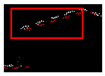
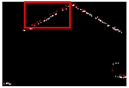
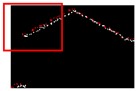
| Before Adjustment Profiles | Proposed Method Profiles | Comparison Method Profile | TerraMatch Profile | ||||
|---|---|---|---|---|---|---|---|
 | 0.353 |  | 0.011 |  | 0.023 |  | 0.013 |
 | 0.358 |  | 0.011 |  | 0.013 |  | 0.023 |
 | 0.423 | 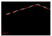 | 0.007 | 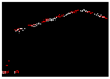 | 0.010 | 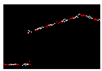 | 0.006 |
 | 0.457 |  | 0.008 |  | 0.007 |  | 0.011 |
 | 0.375 |  | 0.007 |  | 0.010 |  | 0.005 |
 | 0.346 |  | 0.006 |  | 0.006 |  | 0.005 |
 | 0.510 | 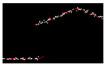 | 0.012 |  | 0.013 | 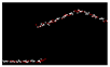 | 0.015 |
 | 0.478 |  | 0.012 |  | 0.011 | 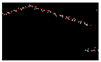 | 0.014 |
| RMSE | 0.417 | - - | 0.010 | - - | 0.013 | - - | 0.013 |
| - - | - - | 97.6% | - - | 96.8% | - - | 96.8% | |
| Serial No. of Adjacent Strips | Number of Corresponding Buildings | Number of Corresponding Roof Planes | (m) |
|---|---|---|---|
| 1 & 2 | 70 | 114 | 0.023 |
| 2 & 3 | 37 | 54 | 0.028 |
| 3 & 4 | 102 | 118 | 0.035 |
| 4 & 5 | 128 | 171 | 0.030 |
| 5 & 6 | 121 | 152 | 0.032 |
| 6 & 7 | 36 | 45 | 0.033 |
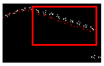
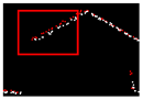
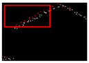
| Before Adjustment Profiles | Adjustment by the Proposed Method Profiles | Adjustment by the Comparison Method Profiles | |||
|---|---|---|---|---|---|
 | 0.212 |  | 0.011 | 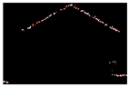 | 0.012 |
 | 0.322 | 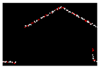 | 0.007 |  | 0.007 |
 | 0.206 |  | 0.011 |  | 0.013 |
 | 0.253 |  | 0.009 |  | 0.011 |
 | 0.197 |  | 0.013 |  | 0.013 |
 | 0.222 |  | 0.008 |  | 0.009 |
 | 0.230 | 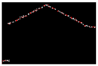 | 0.012 |  | 0.014 |
 | 0.422 | 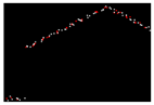 | 0.004 |  | 0.007 |
| RMSE | 0.268 | - - | 0.010 | - - | 0.011 |
| - - | - - | 96.3% | - - | 95.9% | |
© 2019 by the authors. Licensee MDPI, Basel, Switzerland. This article is an open access article distributed under the terms and conditions of the Creative Commons Attribution (CC BY) license (http://creativecommons.org/licenses/by/4.0/).
Share and Cite
Liu, K.; Ma, H.; Zhang, L.; Cai, Z.; Ma, H. Strip Adjustment of Airborne LiDAR Data in Urban Scenes Using Planar Features by the Minimum Hausdorff Distance. Sensors 2019, 19, 5131. https://doi.org/10.3390/s19235131
Liu K, Ma H, Zhang L, Cai Z, Ma H. Strip Adjustment of Airborne LiDAR Data in Urban Scenes Using Planar Features by the Minimum Hausdorff Distance. Sensors. 2019; 19(23):5131. https://doi.org/10.3390/s19235131
Chicago/Turabian StyleLiu, Ke, Hongchao Ma, Liang Zhang, Zhan Cai, and Haichi Ma. 2019. "Strip Adjustment of Airborne LiDAR Data in Urban Scenes Using Planar Features by the Minimum Hausdorff Distance" Sensors 19, no. 23: 5131. https://doi.org/10.3390/s19235131