New Fast Arctangent Approximation Algorithm for Generic Real-Time Embedded Applications

 ,
,  ,
,
Abstract
:1. Introduction
2. Review of Arctangent Approximation Techniques
2.1. Iterative CORDIC
2.2. Lookup Tables (LUT) Techniques
2.3. Rational Approximations
2.4. Approximation Techniques Qualitative Comparison
3. Rational Formulae Comparison
3.1. New 2nd Order Rational Approximation Formula
3.2. Rational Formulae Classification
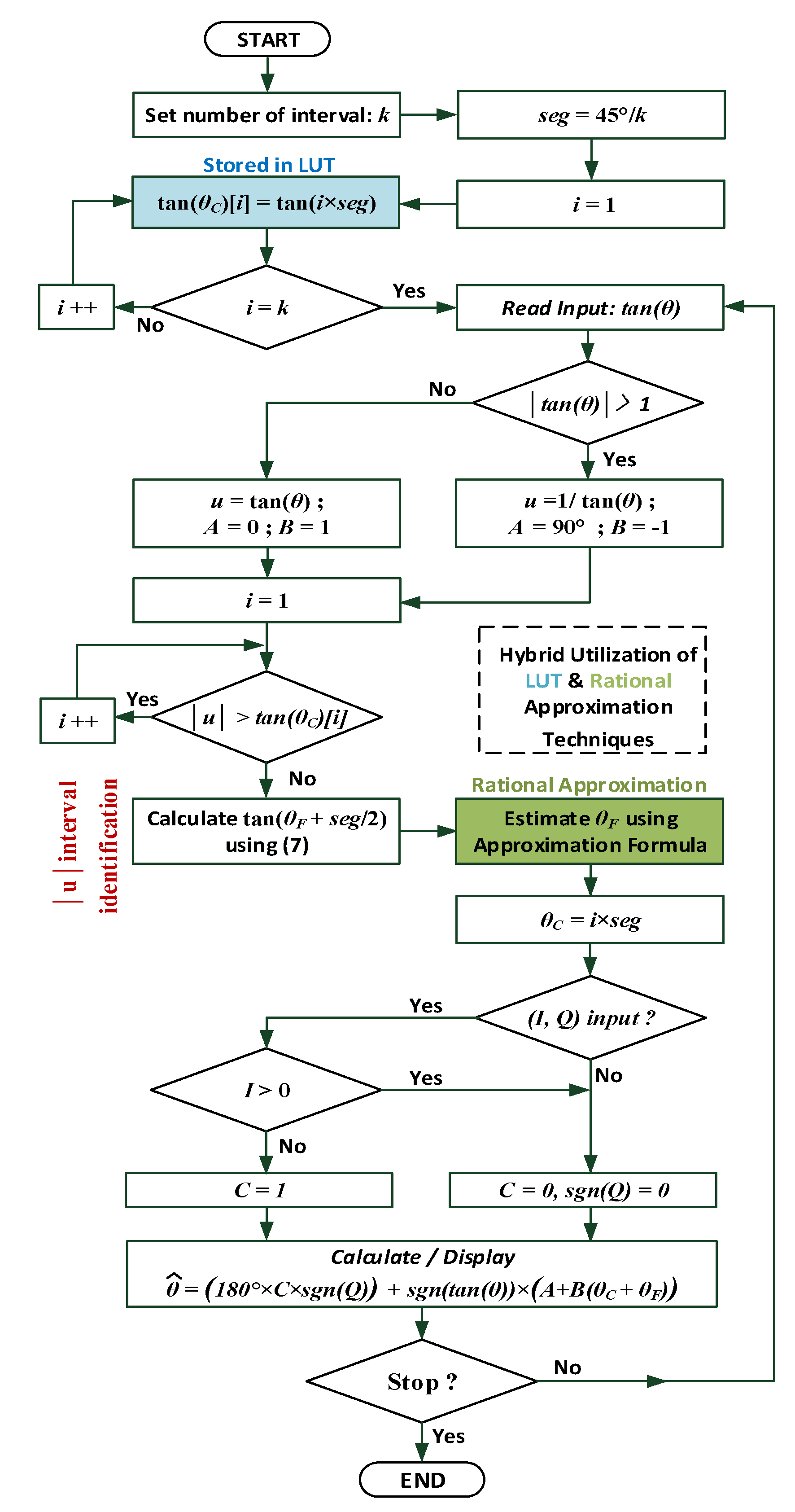
4. Proposed Arctangent Approximation Algorithm
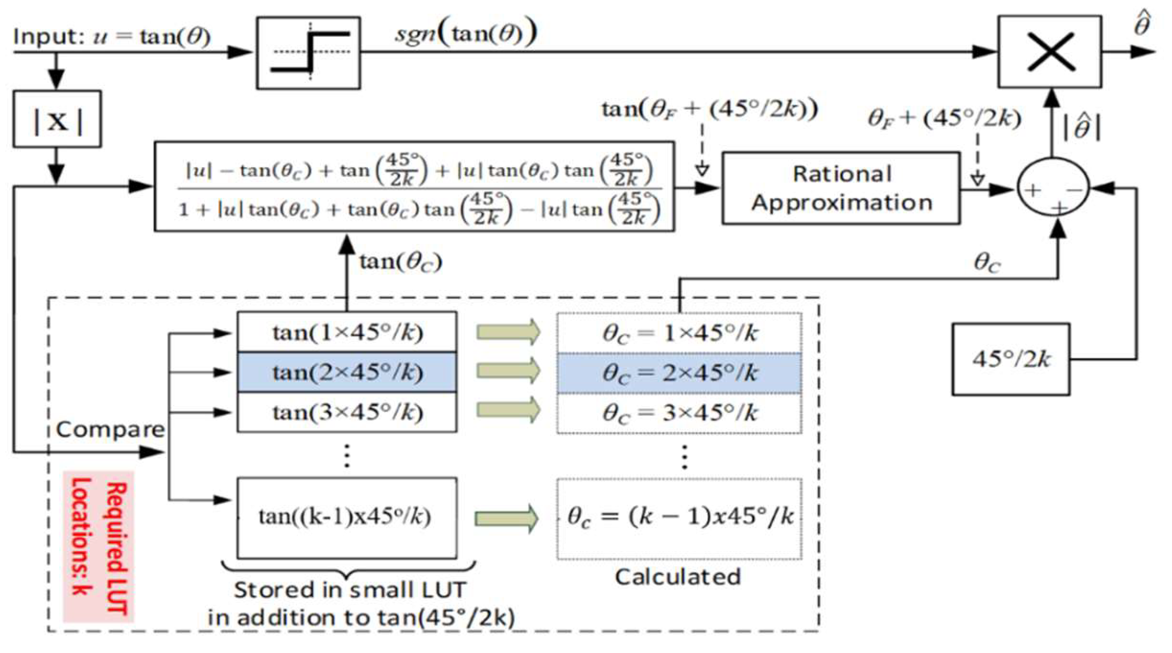
4.1. Step 1: Input Segmentation Methodology ()
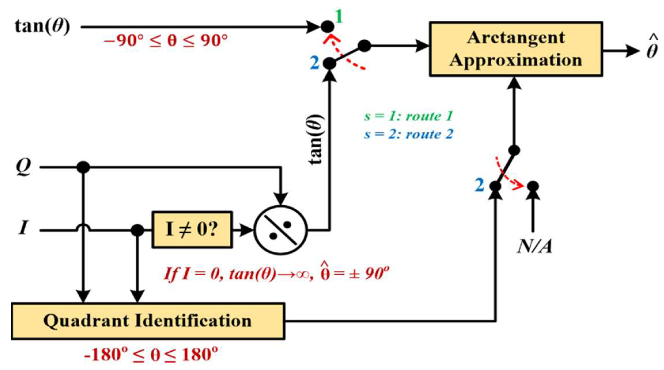
4.2. Step 2: Referring the Input to Its Original 360° Value (Generic Algorithm Application)
5. Proposed Algorithm Validation
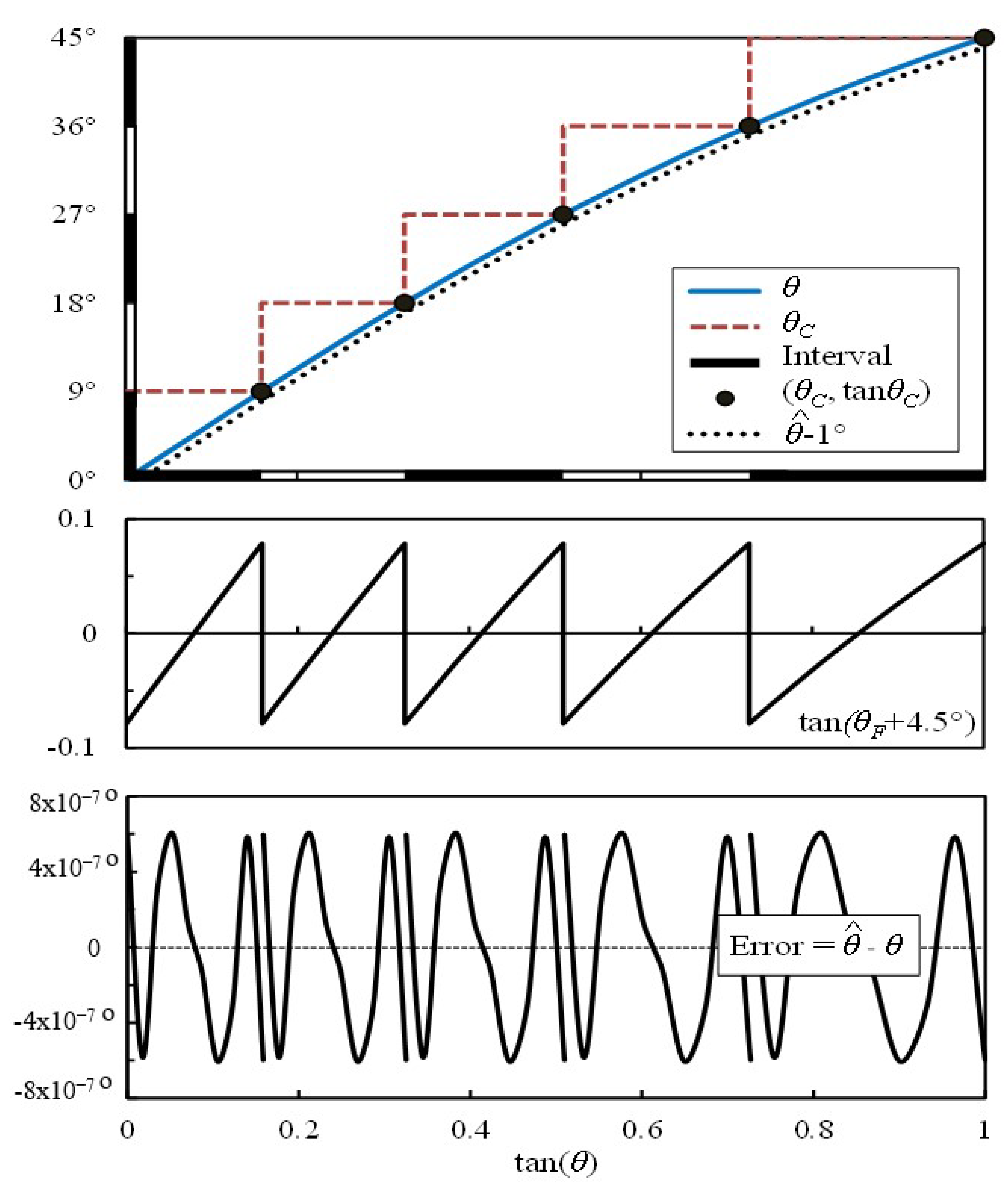
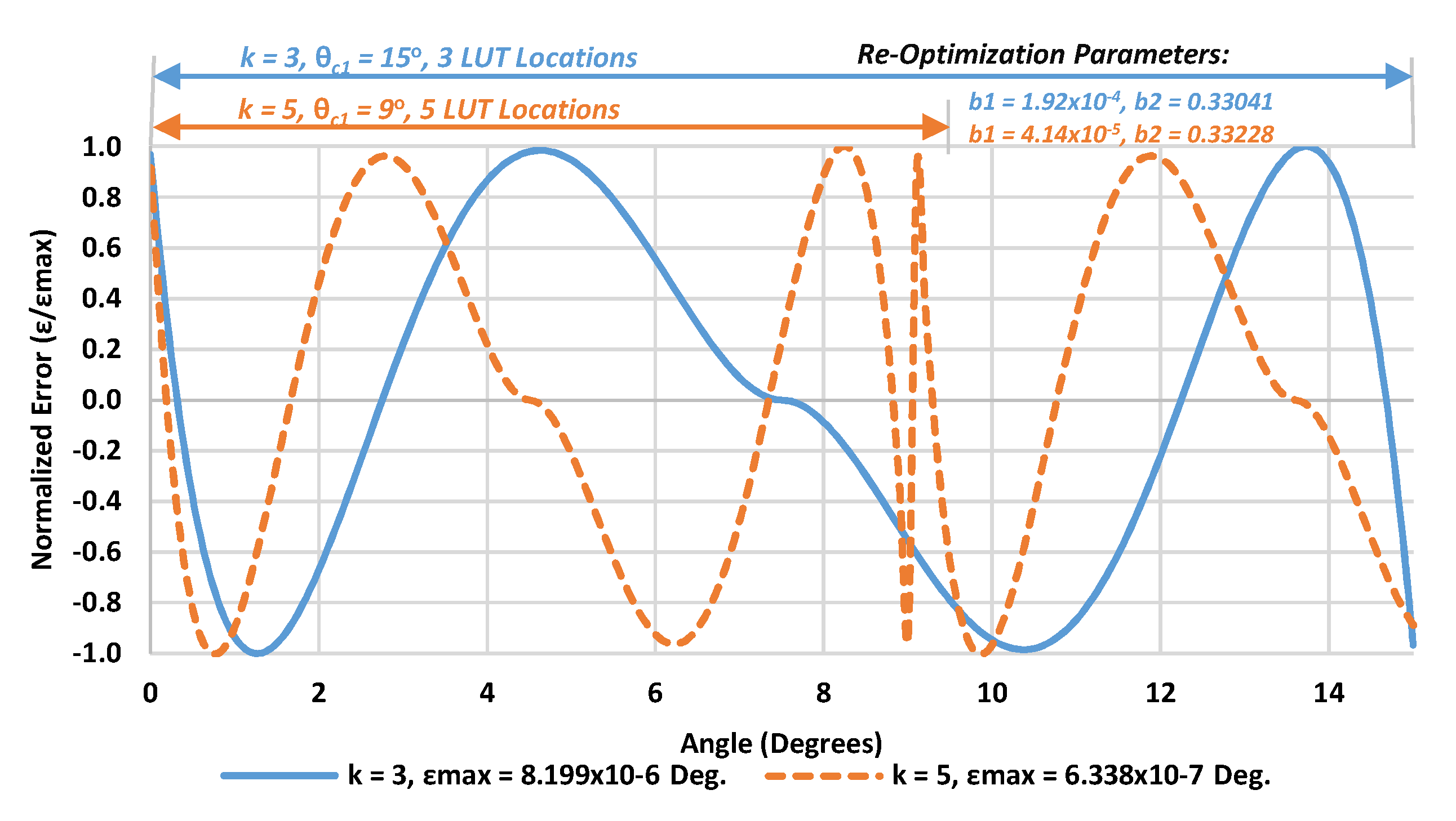
5.1. Interval Size Effect on the New Algorithm Performance
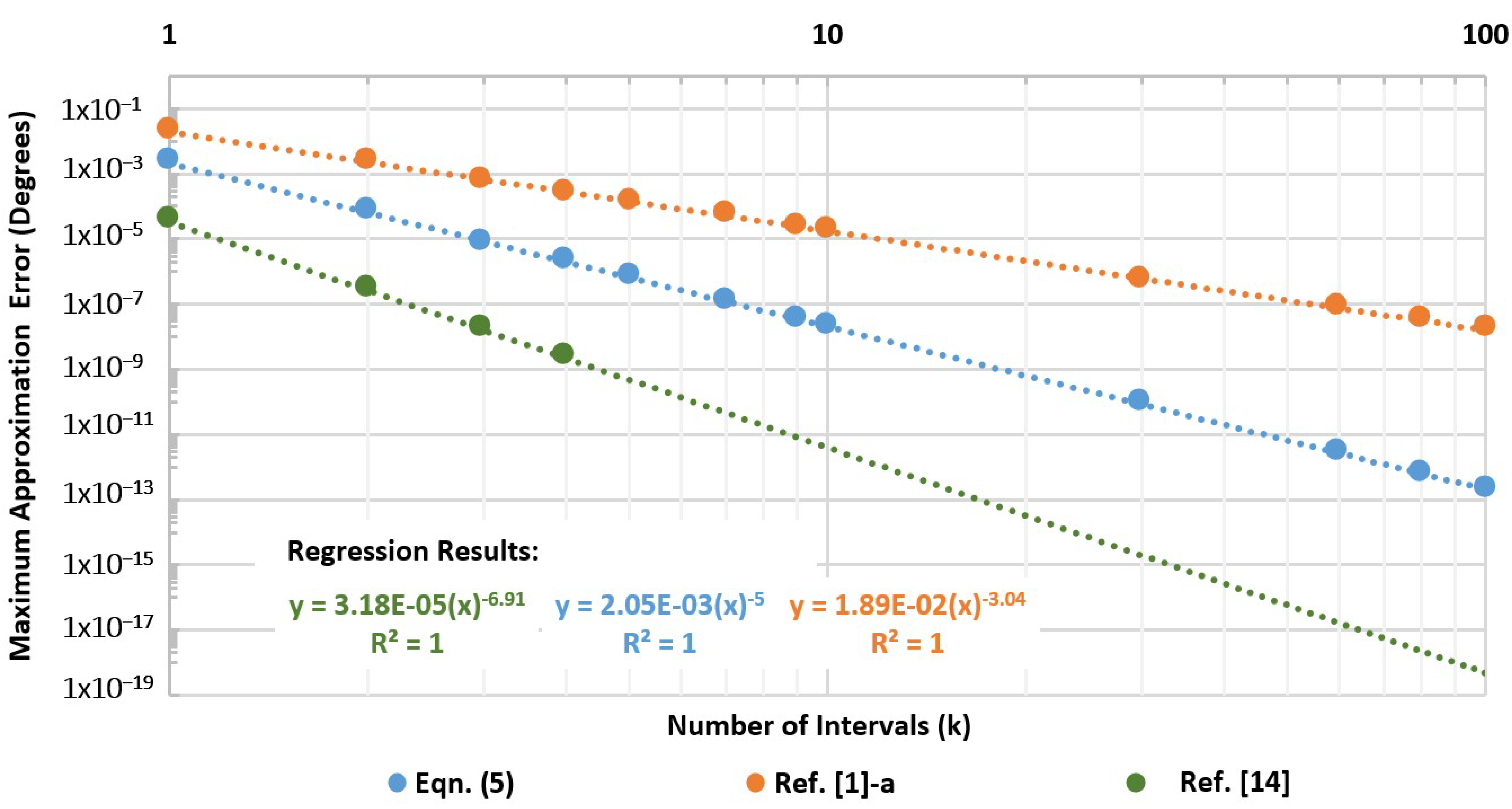
5.2. Performance Comparison of the Three Selected Rational Formulae for Algorithm Implementation
5.2.1. Fourth Order Approximation
5.2.2. Third Order Approximation
5.2.3. Second Order Approximation
5.2.4. Performance Analysis
6. Conclusions
Author Contributions
Funding
Conflicts of Interest
Dedication
References
- Rajan, S.; Wang, S.; Inkol, R. Efficient Approximations for the Arctangent Function. IEEE Signal Process. Mag. 2006, 23, 108–111. [Google Scholar] [CrossRef]
- Ukil, A.; Shah, V.H.; Deck, B. Fast computation of arctangent functions for embedded applications: A comparative analysis. In Proceedings of the 2011 IEEE International Symposium on Industrial Electronics, Gdansk, Poland, 27–30 June 2011; pp. 1206–1211. [Google Scholar]
- Ben-Brahim, L.; Benammar, M.; Alhamadi, M.A. A Resolver Angle Estimator Based on Its Excitation Signal. IEEE Trans. Ind. Electron. 2009, 56, 574–580. [Google Scholar] [CrossRef]
- Wang, L.; Zhang, Y.; Hao, S.; Song, B.; Hao, M.; Tang, Z. Study on high precision magnetic encoder based on PMSM sensorless control. Sens. Rev. 2016, 36, 267–276. [Google Scholar] [CrossRef]
- Benammar, M.; Khattab, A.; Saleh, S.; Bensaali, F.; Touati, F. A Sinusoidal Encoder-to-Digital Converter Based on an Improved Tangent Method. IEEE Sens. J. 2017, 17, 5169–5179. [Google Scholar] [CrossRef]
- Gu, C.; Li, C.; Lin, J.; Long, J.; Huangfu, J.; Ran, L. Instrument-Based Noncontact Doppler Radar Vital Sign Detection System Using Heterodyne Digital Quadrature Demodulation Architecture. IEEE Trans. Instrum. Meas. 2010, 59, 1580–1588. [Google Scholar] [CrossRef]
- Gu, C. Short-Range Noncontact Sensors for Healthcare and Other Emerging Applications: A Review. Sensors 2016, 16, 1169. [Google Scholar] [CrossRef] [PubMed]
- Girones, X.; Julia, C.; Puig, D. Full Quadrant Approximations for the Arctangent Function [Tips and Tricks]. IEEE Signal Process. Mag. 2013, 30, 130–135. [Google Scholar] [CrossRef]
- Pilato, L.; Fanucci, L.; Saponara, S. Real-Time and High-Accuracy Arctangent Computation Using CORDIC and Fast Magnitude Estimation. Electronics 2017, 6, 22. [Google Scholar] [CrossRef]
- Lyons, R. Another contender in the arctangent race. IEEE Signal Process. Mag. 2004, 21, 109–110. [Google Scholar] [CrossRef]
- Torres, V.; Valls, J.; Lyons, R. Fast- and Low-Complexity atan2(a,b) Approximation [Tips and Tricks]. IEEE Signal Process. Mag. 2017, 34, 164–169. [Google Scholar] [CrossRef]
- Rajan, S.; Wang, S.; Inkol, R. Error reduction technique for four-quadrant arctangent approximations. IET Signal Process. 2008, 2, 133–138. [Google Scholar] [CrossRef]
- Torres, V.; Valls, J. A Fast and Low-Complexity Operator for the Computation of the Arctangent of a Complex Number. IEEE Trans. VLSI Syst. 2017, 25, 2663–2667. [Google Scholar] [CrossRef]
- Zarowski, C. Differential Evolution for a Better Approximation to the Arctangent Function, Nanodottek Report NDT3-04-2006. 2006.
- López, A.; Vélez, P.; Moriano, C. Approximations to the magic formula. Int. J. Automot. Technol. 2010, 11, 155–166. [Google Scholar] [CrossRef]
- Ye, G.; Liu, H.; Fan, S.; Li, X.; Yu, H.; Lei, B.; Shi, Y.; Yin, L.; Lu, B. Precise and robust position estimation for optical incremental encoders using a linearization technique. Sensors Actuators A Phys. 2015, 232, 30–38. [Google Scholar] [CrossRef]
- Saber, M.; Jitsumatsu, Y.; Kohda, T. A low-power implementation of arctangent function for communication applications using FPGA. Proceedings of the 2009 Fourth International Workshop on Signal Design and Its Applications in Communications, Fukuoka, Japan, 19–23 October 2009; pp. 60–63. [Google Scholar]

| Technique | Advantages | Limitations |
|---|---|---|
| CORDIC |
|
|
| LUT |
|
|
| Rational |
|
|
| Work | (μs) | ||
|---|---|---|---|
| [14] | 0.0030 | 18.00 | |
| [8] | 0.0081 | 6.60 | |
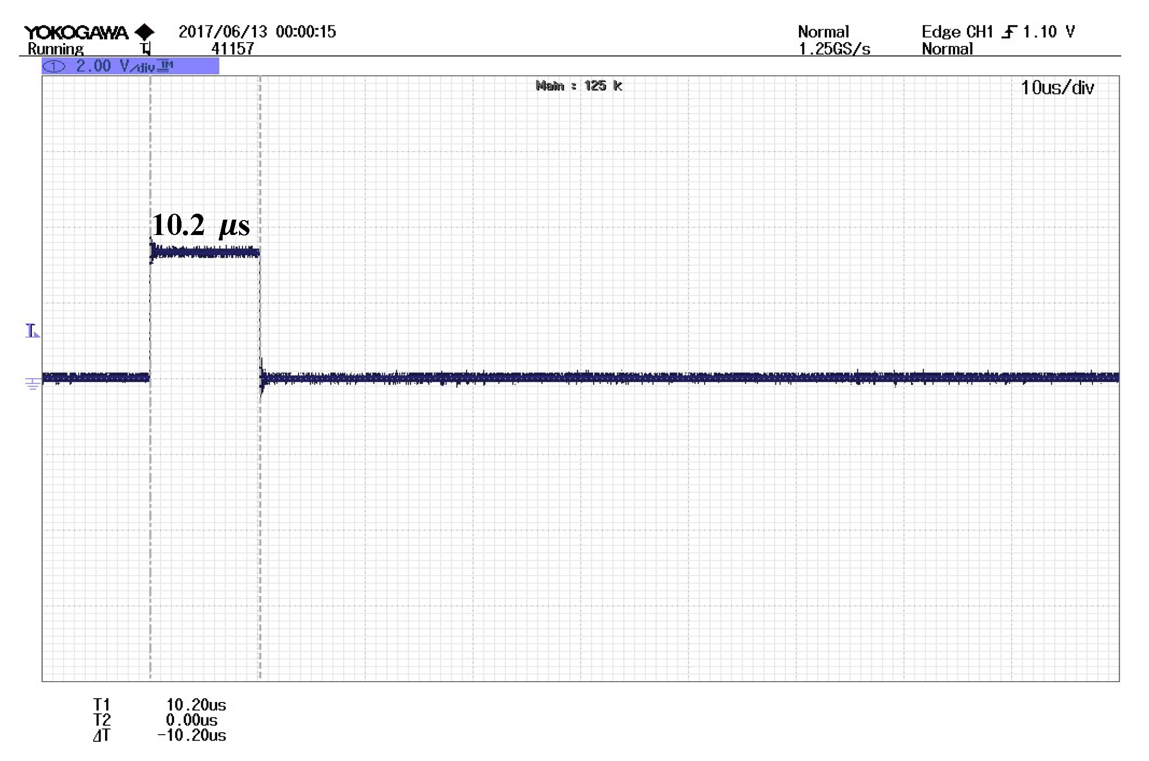
| Present, Equation (5) | 0.0777 | 3.50 | |
| [1]-a * | 0.0862 | 0.57 | |
| [15] | 0.2000 | 3.52 | |
| [1]-b | 0.2138 | 0.54 | |
| [10] | 0.2632 | 3.42 | |
| [1]-c | 0.2833 | 1.91 | |
| [16] ** | 0.3502 | 1.92 |
| i | ||
| 1 | 0.1584 | 9° |
| 2 | 0.3249 | 18° |
| 3 | 0.5095 | 27° |
| 4 | 0.7265 | 36° |
| 5 | 1.0000 | 45° |
| Example of atan (u) Estimation Using Proposed Method with Equation (5). | ||
| Input: | ||
| STEP 1: | ||
| STEP 2: calculate | STEP 3: Estimate using adequate formula, e.g., Equation (5). | |
; | ||
| Range Output: | ||
© 2019 by the authors. Licensee MDPI, Basel, Switzerland. This article is an open access article distributed under the terms and conditions of the Creative Commons Attribution (CC BY) license (http://creativecommons.org/licenses/by/4.0/).
Share and Cite
Benammar, M.; Alassi, A.; Gastli, A.; Ben-Brahim, L.; Touati, F. New Fast Arctangent Approximation Algorithm for Generic Real-Time Embedded Applications. Sensors 2019, 19, 5148. https://doi.org/10.3390/s19235148
Benammar M, Alassi A, Gastli A, Ben-Brahim L, Touati F. New Fast Arctangent Approximation Algorithm for Generic Real-Time Embedded Applications. Sensors. 2019; 19(23):5148. https://doi.org/10.3390/s19235148
Chicago/Turabian StyleBenammar, Mohieddine, Abdulrahman Alassi, Adel Gastli, Lazhar Ben-Brahim, and Farid Touati. 2019. "New Fast Arctangent Approximation Algorithm for Generic Real-Time Embedded Applications" Sensors 19, no. 23: 5148. https://doi.org/10.3390/s19235148