Maize Crop Coefficient Estimated from UAV-Measured Multispectral Vegetation Indices

Abstract

The rapid, accurate, and real-time estimation of crop coefficients at the farm scale is one of the key prerequisites in precision agricultural water management. This study aimed to map the maize crop coefficient (K_c) with improved accuracy under different levels of deficit irrigation. The proposed method for estimating the K_c is based on multispectral images of high spatial resolution taken using an unmanned aerial vehicle (UAV). The analysis was performed on five experimental plots using K_c values measured from the daily soil water balance in Ordos, Inner Mongolia, China. To accurately estimate the K_c, the fraction of vegetation cover (f_c) derived from the normalized difference vegetation index (NDVI) was used to compare with field measurements, and the stress coefficients (K_s) calculated from two vegetation index (VI) regression models were compared. The results showed that the NDVI values under different levels of deficit irrigation had no significant difference in the reproductive stage but changed significantly in the maturation stage, with a decrease of 0.09 with 72% water applied difference. The f_c calculated from the NDVI had a high correlation with field measurement data, with a coefficient of determination (R²) of 0.93. The ratios of transformed chlorophyll absorption in reflectance index (TCARI) to renormalized difference vegetation index (RDVI) and TCARI to soil-adjusted vegetation index (SAVI) were used, respectively, to establish two types of K_s regression models to retrieve K_c. Compared to the TCARI/SAVI model, the TCARI/RDVI model under different levels of deficit irrigation had better correlation with K_c, with R² and root-mean-square error (RMSE) values ranging from 0.68 to 0.80 and from 0.140 to 0.232, respectively. Compared to K_c calculated from on-site measurements, the K_c values retrieved from the VI regression models established in this study had greater ability to assess the field variability of soil and crops. Overall, use of the UAV-measured multispectral vegetation index approach could improve water management at the farm scale.

1. Introduction

Water scarcity is a major factor limiting irrigated agriculture, especially in arid and semi-arid areas of the world. Due to global climate changes and the imbalance between water supply and demand, it is particularly necessary to improve crop water use [1]. Therefore, the regulated deficit irrigation (RDI) strategy for reducing water consumption is widely used in current agriculture [2]. In this context, how to accurately estimate and monitor crop water requirements is not only the key for optimizing irrigation scheduling and improving water use efficiency, but also essential research for enhancing food production and SAVIng regional water resources [3,4].

A common indicator of crop water requirements is the crop coefficient (K_c), which was presented in FAO 56 [5] and is used to estimate crop evapotranspiration (ET_c) by multiplying the reference crop evapotranspiration (ET₀) [6]. The K_c primarily depends on meteorological information, crop-specific coefficients, the lengths of crop growth stages, and plant-available soil water [7]. It can be estimated using single and dual K_c approaches. The single approach is the averaging of K_c trends that incorporate plant transpiration (K_cb) and soil evaporation (K_e). Compared to the single approach, the dual approach improves the estimation accuracy of ET by considering the plant transpiration and soil evaporation separately, i.e., K_c = K_cb + K_e [8]. However, in practical crop conditions, the K_c needs to be appropriately adjusted by using a stress coefficient (K_s) for nonstandard conditions, especially water stress conditions [6]. The dual approach has been appropriately used for crops at a field or regional scale [9,10,11,12,13].

To date, several methods have been presented to monitor K_c, such as soil water balance, eddy covariance, Bowen ratio, lysimeter, and remote sensing [14,15,16,17,18]. In situ measurements are likely to be time-consuming and costly, and make it hard to consider the spatial variability of crops and soil [19]. Therefore, remote sensing of K_c has become increasingly recommended in irrigation management. One of the most common approaches is to estimate the real-time K_cb and K_c through empirical equations of vegetation indices (VIs) such as the normalized difference vegetation index (NDVI) derived from multispectral images [20,21,22,23]. Such empirical equations rely on the close relationship between the VIs and various actual plant growth parameters, e.g., leaf area index [24,25], fraction of ground covered by plants [26,27], and biomass [24,28]. However, Pereira et al. [7] noted that NDVI-based methods can not accurately observe a decrease in K_c and K_cb when crops are under water stress. Zhang and Zhou [29] proposed that crop water status can be accurately monitored using the VIs which are not only sensitive to water information but also contain vegetation growth status. Consequently, partial VIs such as the reflectance index (TCARI), optimization of soil-adjusted vegetation index (OSAVI), soil-adjusted vegetation index (SAVI), and renormalized difference vegetation index (RDVI) can effectively monitor crop water status [30]. For example, Haboudane et al. [31] utilized TCARI/OSAVI to predict maize water status in Canada and reported a high correlation between TCARI/OSAVI and chlorophyll content. Zhang et al. [19] evaluated maize water stress and its spatial variability by multispectral remote sensing. The results showed that two regression models based on TCARI/RDVI and TCARI/SAVI were able to monitor the crop water stress index (CWSI) with respective coefficients of determination (R²) of 0.81 and 0.80 under different levels of deficit irrigation.

Unmanned aerial vehicles (UAVs) in remote sensing have exponentially increased in applications of precision agriculture over the past decade [32]. Compared to conventional data acquisition methods for remote sensing, such as satellites and spectrometers [33,34], UAVs offer many obvious advantages to support water resource management and planning [35,36]. One of the most common advantages is that UAVs can provide high-quality data at the required scale and time, while conventional methods have not been applied in practice at the farm scale due to their coarse spatial resolution, infrequent coverage, and high cost [37,38]. Additionally, UAVs can be used to obtain low-cost data as frequently as necessitated by the monitoring task because of their ease of operation and deployment, their high flexibility, and the decreasing cost of the platform [39]. Thus, UAV-based monitoring has become increasingly pervasive in supporting the real-time control of irrigation systems.

In recent works, the abovementioned K_s has usually been calculated using the FAO-56 soil water depletion method proposed by Allen et al. [5]. For example, Pôças et al. [6] estimated the actual K_c for maize, barley, and olive based on VIs and a soil water balance model under water stress conditions. The results showed that the K_s computed using the soil water balance model could accurately exhibit reductions in K_c due to water stress. Another method to determine K_s is based on indications of the infrared canopy temperature, such as the CWSI. Kullberg et al. [40] compared the performance of several canopy temperature methods converted into K_s. The results showed that the CWSI based on infrared thermal radiometry (IRT) had the best accuracy compared to other methods, and it is typically considered to be scalable to K_s. Bellvert et al. [41] stated that mapping CWSI from UAV thermal imagery has the limitation of inevitable mixed temperatures coming from both the soil and leaves due to bigger pixels and full cover. Considering the relationship between VIs and the CWSI discussed above, VIs have been found to have a comparable ability to monitor K_c under water stress conditions. However, research using VIs derived from a UAV multispectral remote sensing system is still relatively rare in K_c estimation at the farm scale under different levels of water stress.

Therefore, in this study, we established a K_c empirical model based on UAV multispectral remote sensing to represent the crop evapotranspiration of summer maize under different levels of deficit irrigation. The main objectives were as follows:

(1) To explore the differences in K_c with regard to the soil water balance in response to water stress treatments at different growth stages;

(2) To establish K_c regression models based on UAV multispectral VIs that are sensitive to maize water stress and compare them with measured crop coefficients;

(3) To obtain K_c maps derived from the K_c regression model with high spatial–temporal resolution at the farm scale.

2. Materials and Methods

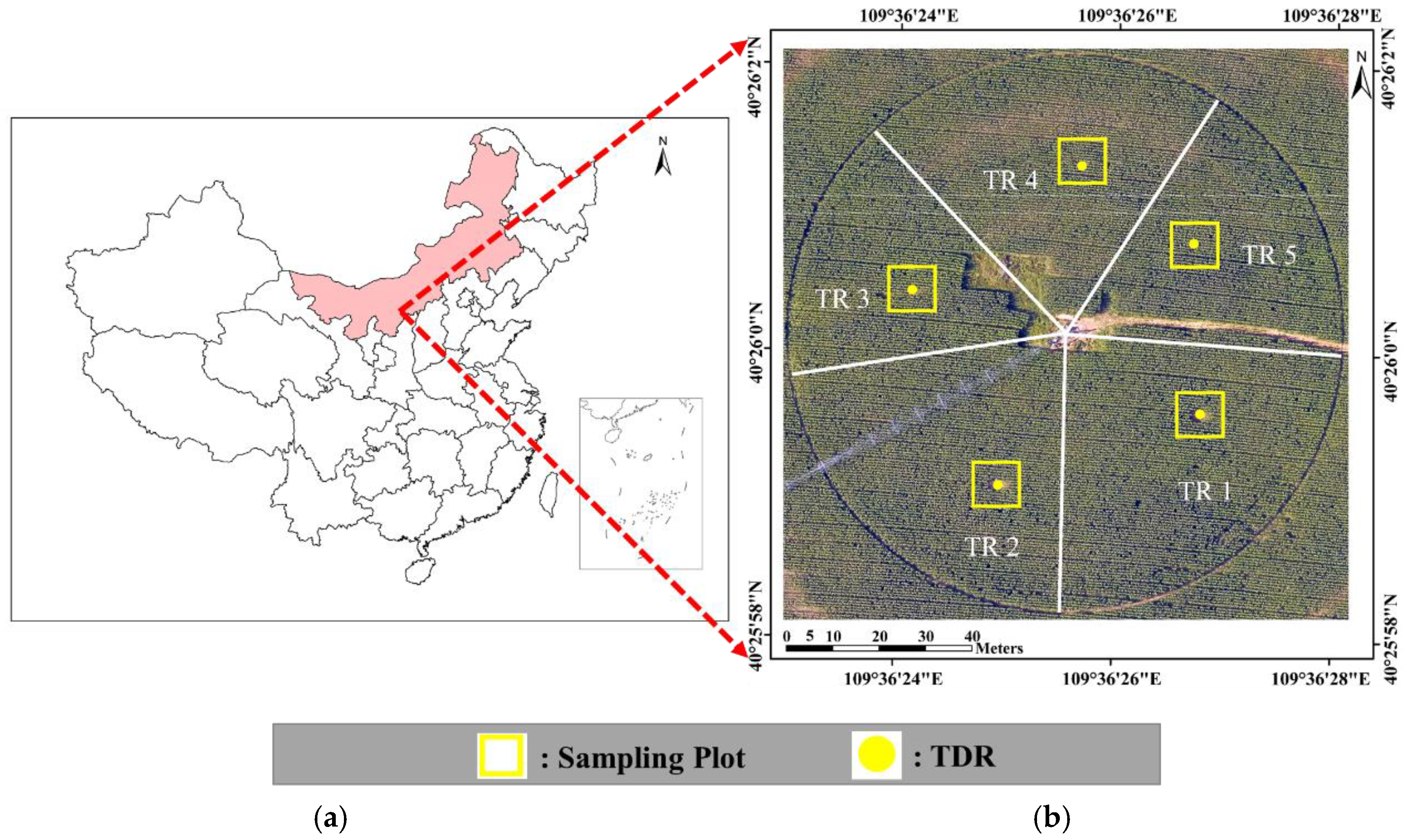
2.1. Study Area

The study was carried out on an experimental farm located in Zhaojun Town, southwest Inner Mongolia, China (40°26′0.29” N, 109°36′25.99” E). The experimental area is approximately 1.13 ha at 1010 m altitude above the sea level. The climate is semi-arid, and the soil type is loamy sand with 80.7% sand, 13.7% powder, and 5.6% clay. The average field capacity (0–90 cm soil depth) is 0.169 m³·m⁻³, and the average soil bulk density is 1.56 g·cm⁻³. The soil pH, C content, and organic matter are 9.27, 27.35 g/Kg, and 47.17 g/Kg, respectively. Maize (Junkai 918) was sowed on 20 May 2017 (day of year (DOY) 140), with a 0.58 m planting distance and 0.25 m plant spacing, and the row direction was from east to west. The maize emerged on 1 June, headed on 20 July, and was harvested on 7 September (silage), giving a 110-day lifespan [19].

2.2. Experimental Design

There were five different levels of deficit irrigation treatments for which we divided the study field into treatment (TR) regions (Figure 1b). In order to effectively collect data and control irrigation water, a 12 × 12 m² experimental plot was chosen in each treatment region. The five treatments were full irrigation (TR1), slight water stress (TR5), moderate water stress (TR2 and TR3), and severe water stress (TR4). TR1 represented the total crop water requirement of fully watered maize during the whole growth period. The different levels of deficit irrigation were designed according to the percentages of applied water depth of TR1 during the late vegetation, reproductive, and maturation stages. For example, during the maturation stage, 52% of the applied water depth at TR1 was applied to TR2 (

Table 1. Experimental treatments and total applied water depth (percentage of full irrigation treatment in parentheses) that includes the amount of irrigation and precipitation in the late vegetative, reproductive, and maturation stages in 2017 (taken from Zhang et al. [19]).

Treatment	Applied Water Depth/mm
	Late Vegetative (06.20–07.28)	Reproductive (07.29–08.20)	Maturation (08.21–09.07)	Total
TR 1	188 (100%)	132 (100%)	82 (100%)	402
TR 2	158 (84%)	128 (97%)	43 (52%)	329
TR 3	158 (84%)	125 (95%)	43 (52%)	326
TR 4	158 (84%)	91 (69%)	23 (28%)	272
TR 5	158 (84%)	124 (94%)	82 (100%)	365

).

A central pivot sprinkler system (Valmont Industries, Inc., Omaha, NE, USA) was used for irrigation, and different irrigation amounts were processed in each treatment region by adjusting the speed of the sprinkler system. The test for water application uniformity of the central pivot irrigation system was carried out in accordance with the standards ANSI/ASAE S436.1 and ISO 11545. The uniformity coefficient for the first span (research area) of the R3000 sprinklers was calculated using the modified formula by Heermann and Hein [42], and the values were 82.7% and 88.3% under 20% and 40% of full walking speed, respectively. The amount of water applied to each treatment was measured and recorded using a MIK-2000H flow meter (Meacon Automation Technology co., Ltd., Hangzhou, China). Due to the influence of rainfall, the actual applied water depth (irrigation and rainfall amount) for each growth stage in each treatment region is shown in Table 1. In order to eliminate the stress of nutrients and weeds, fertilizer and herbicide were applied according to planting experience.

In order to obtain daily data on the soil water content, each of the five experimental plots was installed with a monitoring station with a time domain reflectometry (TDR) probe (TDR 315L, Acclima, Inc., Boise, ID, USA). The distribution of voltage pulses was done around a coaxial cable of length 3 m, and this cable was connected to a TDR 315L probe (0.15 m in length). Access tubes were installed vertically up to 90 cm into the soil in the middle of each plot, and the probe was inserted into the soil to access the tubes at different depths (30, 60, 90 cm) for the measurement of the daily volumetric soil water content (SWC) during the study period.

2.3. Meteorological Data

The weather data were recorded by an automated weather station located at a farm adjacent to the research field. The daily and hourly measured weather variables included rainfall, air temperature and relative humidity, net solar radiation, and wind speed (2 m above the reference grass surface). The main mean meteorological data during the study period, including the late vegetative stage (06.26–07.28), reproductive stage (07.29–08.20), and maturation stage (08.21–29), are shown in

Table 2. The main mean meteorological data during the study period, including the late vegetative stage, reproductive stage, and maturation stage in 2017.

Parameter	Late Vegetative (06.26–07.28)	Reproductive (07.29–08.20)	Maturation (08.21–29)
Mean air temp./°C	24.33	22.11	17.21
Max air temp./°C	37.30	31.31	25.46
Min air temp./°C	11.70	13.61	9.24
Min relative humidity/%	19.41	29.78	33.23
Mean net solar radiation/MJ·m−2·day−1	13.08	10.98	3.00
Mean wind speed/m·s−1	0.66	0.47	0.28
Rainfall/mm	2.8	38.8	2.8

.

2.4. Crop Coverage Measurement

A DJI Phantom 4 Pro with an 84° field of view lens, an f/2.8 aperture, and a resolution of 4864 × 3648 pixels was used to obtain crop coverage (f_c). The flights were conducted every 3 to 7 days between 11:00 and 13:00 local time, at 50 m altitude, and with a ground sample distance of 1.4 cm. The overlap of imagery to the front and side was 80%. The mosaic RGB images were acquired using Pix4DMapper software (Lausanne, Switzerland). The RGB images of each sampling plot were classified into soil and vegetation using supervised classification aided by ENVI 5.3 software. The f_c value was derived as the percentage detected as vegetation.

2.5. Soil Water Balance

The daily crop evapotranspiration (ET_c) was obtained using the soil water balance equation with soil water content measured by TDR [5,43,44,45] (Equation (1)):

$$E{T}_c=P+I\pm \Delta SM-D_p-RO+CR$$

(1)

where ET_c represents crop evapotranspiration; P represents the precipitation; I represents the irrigation; ΔSM represents the change in water content between two successive days, calculated by TDR; DP represents deep percolation; RO represents surface runoff; and CR represents capillary rise from the deep water table, which can be ignored due to the shallow to deep water table depth (3–55 m) and also due to no contribution from groundwater with capillary rise into the root zone [46]. All terms in the soil water balance are in millimeters. An example of the results of the changing curve of the average SWC (volumetric) at the depths of 30, 60, and 90 cm at TR1 during the study period is shown in Figure 2.

2.6. UAV Multispectral Imagery Acquisition

A multispectral camera (RedEdge, MicaSense, Inc., Seattle, WA, USA) was installed on a UAV platform (a six-rotor unmanned aircraft S900, manufactured by DJI). The S900 six-rotor UAV has the advantages of stable flight and takeoff, strong wind resistance, and low cost. The maximum take-off weight is 6 kg, the maximum payload is 2 kg, the maximum wind speed it can withstand is 5 m/s, and its flight time is 18 min. The RedEdge multispectral camera consists of five bands in the VIS–NIR spectral range at 475, 560, 668, 717, 840 nm, respectively; a 5.5 mm fixed lens; image resolution of 1280 × 960 pixels; and angle of view of 47.2° (H). The flight control board used was a Pixhawk autopilot (CUAV, Guangzhou, China), and the ground control station software Mission Planner was used to conduct the flight planning.

UAV multispectral data from fourteen flights were acquired at a 70 m flight height with 4.7 cm spatial resolution during the study period (2017.06.26~08.29) between 11:00 and 13:00 local time. The heading and side overlap and speed of the UAV were 80% and 5 m/s, respectively. The mosaic multispectral images were acquired using the photogrammetric software Pix4DMapper (Lausanne, Switzerland). In order to calibrate the multispectral images, a diffuse reflector (reflectivity 58%, size 3 × 3 m, Group VIII, Seattle, WA, USA) was used during the data collection. The measured image radiances were later converted to reflectance values to obtain spectral reflectance images.

2.7. The Vegetation Index Approach for Crop Coefficient Estimation

In the present study, the calculation of K_c was made based on the dual crop coefficient approach. This approach divides the total crop coefficient into crop transpiration (K_cb) and soil evaporation (K_e) fractions [47,48]. The K_c can be calculated as follows:

$$K_c=K_{cb}+K_e$$

(2)

where K_cb values were estimated based on NDVI measurements developed in a modified approach by Er-Raki et al. [49], who used 1.07 as the K_cb,max value for durum wheat in a semi-arid climate in Morocco. In our study, we used 1.15 in Equation (3) as the K_cb,max value for maize according to Allen et al. [5]. In addition, K_e values were calculated from the fraction of vegetation cover (f_c), which is strongly related to the NDVI [50]. Therefore, K_cb and K_e in the NDVI approach were derived as [5,51] follows:

$$K_{cb}=1.15\ast (1-(NDV{I}_{max}-NDVI)/(NDV{I}_{max}-NDV{I}_{min}))$$

(3)

$$K_e=0.9\ast (1-f_c)$$

(4)

$$f_c=1.19\ast (NDVI-NDV{I}_{min})$$

(5)

where NDVI_max and NDVI_min are the maximal and minimal measured NDVI values during the growing period. We took values of 0.88 for NDVI_max and 0.14 for NDVI_min according to the UAV map. The value 0.9 in Equation (4) was determined according to FAO 56 [5] based on the observed frequency of irrigation and rainfall. The value 1.19 in Equation (5) was determined according to González-Piqueras et al. [51], based on the f_c being less than 80% for maize.

However, the above formulas represent potential crop evapotranspiration conditions. When water stress occurs, the stress coefficient K_s should be considered. K_s (0 ≤ K_s ≤ 1) is defined as the ratio of actual evapotranspiration (ET_a) to potential evapotranspiration (ET_p), proposed by Allen et al. [5]. The K_s can be calculated as follows:

$$K_s=E{T}_a/E{T}_p=K_c{}_{act}/K_c.$$

(6)

Based on the principle of energy balance, Jackson et al. [52] derived a calculation model for the crop water stress index (CWSI) depending on the canopy temperature. The model establishes the relationship between K_s and CWSI as

$$CWSI=1-E{T}_a/E{T}_p=1-K_s.$$

(7)

Additionally, CWSI can be estimated by two VI regression models proposed by Zhang et al. [19] under different levels of deficit irrigation.

$$CWSI-1=\{\begin{array}{cc}0\hfill & (TCARI/RDVI\le 0.195)\hfill \\ 2.41\ast (TCARI/RDVI)-0.47\hfill & (0.195<TCARI/RDVI<0.609)\hfill \\ 1\hfill & (0.609\le TCARI/RDVI)\hfill \end{array}$$

(8)

$$CWSI-2=\{\begin{array}{cc}0\hfill & (TCARI/SAVI\le 0.182)\hfill \\ 2.46\ast (TCARI/SAVI)-0.45\hfill & (0.182<TCARI/SAVI<0.589)\hfill \\ 1\hfill & (0.589\le TCARI/SAVI)\hfill \end{array}$$

(9)

Therefore, in relation to K_s and actual K_c (K_{c act}), K_s and K_{c act} are derived as follows:

$$K_{cact}=K_s\ast K_c=(1-CWSI)\ast (K_{cb}+K_e).$$

(10)

Combining all the above formulas, two different models for K_c estimation can be finally obtained as follows.

$$K_c-1=\{\begin{array}{c}1.15\ast (1-(NDV{I}_{max}-NDVI)/(NDV{I}_{max}-NDV{I}_{min}))\hfill \\ +0.9\ast (1-1.19\ast (NDVI-NDV{I}_{min}))(TCARI/RDVI\le 0.195)\hfill \\ (1.47-2.41\ast (TCARI/RDVI))\ast (1.15\ast (1-(NDV{I}_{max}-NDVI)/(NDV{I}_{max}-NDV{I}_{min}))\hfill \\ +0.9\ast (1-1.19\ast (NDVI-NDV{I}_{min})))(0.195<TCARI/RDVI<0.609)\hfill \\ 0(0.609\le TCARI/RDVI)\hfill \end{array}$$

(11)

$$K_c-2=\{\begin{array}{c}1.15\ast (1-(NDV{I}_{max}-NDVI)/(NDV{I}_{max}-NDV{I}_{min}))\hfill \\ +0.9\ast (1-1.19\ast (NDVI-NDV{I}_{min}))(TCARI/SAVI\le 0.182)\hfill \\ (1.45-2.46\ast (TCARI/SAVI))\ast (1.15\ast (1-(NDV{I}_{max}-NDVI)/(NDV{I}_{max}-NDV{I}_{min}))\hfill \\ +0.9\ast (1-1.19\ast (NDVI-NDV{I}_{min})))(0.182<TCARI/SAVI<0.589)\hfill \\ 0(0.589\le TCARI/SAVI)\hfill \end{array}$$

(12)

2.8. Vegetation Index Calculations

To establish a regression model between UAV-measured multispectral VIs and K_c, NDVI, TCARI/RDVI, and TCARI/SAVI were used in this study. Their calculation formulas are as follows:

$$NDVI=\frac{{\rho }_{nir}-{\rho }_{red}}{{\rho }_{nir}+{\rho }_{red}}$$

(13)

$$RDVI=\frac{{\rho }_{nir}-{\rho }_{red}}{\sqrt{{\rho }_{nir}+{\rho }_{red}}}$$

(14)

$$SAVI=\frac{(1+0.5)\ast ({\rho }_{nir}-{\rho }_{red})}{{\rho }_{nir}-{\rho }_{red}+0.5}$$

(15)

$$TCARI=3\left[({\rho }_{rededge}-{\rho }_{red})-0.2({\rho }_{rededge}-{\rho }_{green})\ast ({\rho }_{rededge}/{\rho }_{red})\right]$$

(16)

where ${\rho }_{nir}$, ${\rho }_{red}$, ${\rho }_{rededge}$, and ${\rho }_{green}$ are the reflectance values of ground objects in the near-infrared, red, red-edge, and green bands. For statistical analysis, the R programming language (R-3.4.3, https://www.r-project.org/) and the lm() function were used. The coefficient of determination (R²) and root-mean-square error (RMSE) were used as evaluating indicators.

3. Results

3.1. NDVI and the Fraction of Vegetation Cover of Maize

It was observed that the NDVI values under different levels of deficit irrigation did not significant differ in the reproductive stage but changed significantly in the maturation stage, with a decrease of 0.09 in TR4 compared to TR1. The results of f_c calculated from the NDVI (f_{c NDVI}; Equation (5)) were compared with f_c based on field measurement (f_{c field}) for the maize (Figure 3b). Both f_c values showed good agreement for all treatments, with an R² value of 0.93 and regression coefficient b close to 1.0.

3.2. The K_c of Maize

Finally, the K_c values were obtained by using the soil water balance model in the sampling plots. Figure 4 depicts the daily changes in K_c for each deficit irrigation treatment during 2017.06.26~2017.08.29. K_c increased after irrigation/rainfall, reaching a maximum around DOY 205, and then slowly decreased, responding well to irrigation/rainfall events. The K_c values for the different levels of deficit irrigation treatments in the late vegetative, reproductive, and maturation stages had a clear numerical gradient. For example, the average K_c values in the late vegetative stage were low, while the average K_c values in the reproductive stage were maintained at a high level, and the average K_c values in the maturation stage slowly decreased. In addition, the K_c values for the different levels of deficit irrigation treatments were significantly different. For example, compared with TR1 in the reproductive and maturation stages, the K_c value was significantly decreased for TR4 in the reproductive and maturation stages.

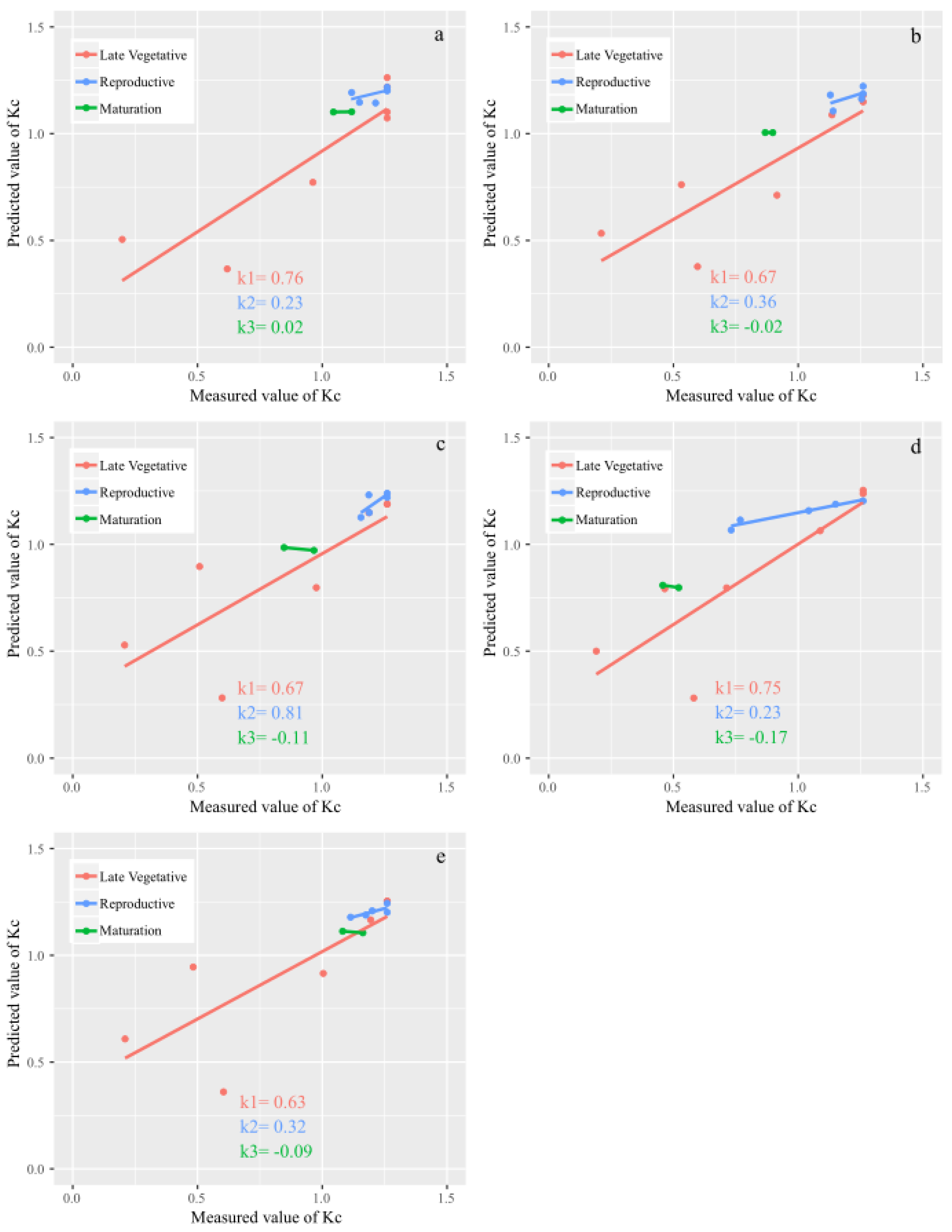
3.3. Estimation of K_c Using Two Different Methods

The results of K_c estimated using the model in Equation (11) (K_c-1) were compared with those from the model in Equation (12) (K_c-2) for the maize under different treatments (

Table 3. Coefficient of determination (R²) and root-mean-square error (RMSE) values from two different predictions of K_c. Values were calculated using Equation (11) (K_c-1) and Equation (12) (K_c-2).

Treatment	Kc-1		Kc-2
	R2 (n = 14)	RMSE	R2 (n = 14)	RMSE
TR 1	0.80 ***	0.140	0.79 ***	0.177
TR 2	0.78 ***	0.150	0.79 ***	0.221
TR 3	0.71 ***	0.174	0.72 ***	0.223
TR 4	0.68 ***	0.232	0.73 ***	0.322
TR 5	0.70 ***	0.180	0.70 ***	0.241

*** p < 0.001.

). The K_c values derived via the two different methods showed a good fit, and their coefficients of determination R² varied from 0.68 to 0.80. The RMSE values were small, within the range of 0.140 to 0.322, indicating adequate stability and fairly tight dispersion in the datasets. However, when the water stress was more serious, both the R² and RMSE were decreased. For example, for K_c-1 with 32% water applied difference between TR1 and TR4, the R² and RMSE values were 0.80 and 0.140 and 0.68 and 0.232, respectively. Compared with the K_c-2 values, the K_c-1 values had better performance as determined by the R² and lower RMSE in all treatments. Therefore, the K_c-1 model was chosen to establish the relationship between the VIs and K_c.

3.4. Crop Coefficient Maps Based on UAV Multispectral Remote Sensing Imagery

Equation (11) was used to retrieve maize crop coefficient maps (Figure 5) based on UAV multispectral remote sensing imagery for DOY 179, 215, 231, and 240. The K_c values of maize under each irrigation treatment showed no significant differences at DOY 179 and DOY 215. In addition, the K_c status of maize under each irrigation treatment showed spatial variations at DOY 231 and DOY 240.

4. Discussion

UAV multispectral technology has been widely used in precision agriculture, but there are also some challenges that need to be solved in the rapid, accurate, and economical estimation of crop coefficients [32,53,54]. Previous studies have observed a high correlation between crop coefficients and VIs obtained from multispectral images, especially NDVI [23,55,56,57]. For example, Mutiibwa and Irmak [58] qualified the effectiveness of using AVHRR-NDVI data to estimate K_c based on a regression model for the U.S. High Plains and showed a good prediction accuracy with an R² value of 0.72 and an RMSE of 0.12. In another study, Kamble et al. [59] derived K_c values from MODIS-NDVI data using a simple linear regression model, resulting in an R² of 0.91 and an RMSE of 0.16.

Previous studies have also reported NDVI-based K_c being successfully applied in many crops, such as maize [60,61,62,63], wheat [15,64], olive orchards [63,65], barley [63,66], sunflower [64], etc. For example, Pôças et al. [64] proposed a combined approach based on NDVI for maize, barley, and olive orchards and showed adequate results for supporting irrigation management. Calera et al. [33] and Cuesta et al. [66] validated NDVI-based K_c values based on a regression model in Castilla La Mancha regions for barley and sunflower irrigated using sprinklers.

However, most studies have established the relationship between K_c and VIs for nonstressed conditions or for conditions of a dry soil surface, which cannot appropriately depict the actual conditions of crop management [6]. Crop coefficients derived from VIs often do not consider the abovementioned K_s, which should be used to obtain the actual K_c under water or salinity stress [7,21]. Stagakis et al. [67] found that most optical indices such as NDVI are suitable for tracking the effects of long-term water stress on crops, while they are not useful as indicators to detect and monitor early water stress conditions. In this work, we also found that the NDVI values under different levels of deficit irrigation did not significantly differ in the reproductive stage, but they changed significantly in the maturation stage, with a decrease of 0.09 in TR4 compared to TR1 (Figure 3a). This is because crops may prevent damage through photo-protection strategies to reduce the leaf absorbance and reflectance changes during short-term water stress [68]. Moreover, crops consume extra energy by reducing chlorophyll b and interconverting xanthophyll cycle pigments [69]. Therefore, previous studies found that VIs are prone to reflecting the chlorophyll and xanthophyll content, which are commonly used to monitor crop water stress status. For instance, Baluja et al. [70] assessed vineyard water status by TCARI/OSAVI with R² values of 0.58 and 0.84 (n = 10) when compared to stem water potential and stomatal conductance, respectively. Here, the CWSI based on regression models was used to obtain K_s from UAV multispectral orthomosaic images, and two CWSI estimation methods were derived from TCARI/RDVI and TCARI/SAVI. These two indices were designed to detect crop water stress status in a more robust and adequate manner. In a relevant study by Zhang et al. [19], TCARI/RDVI and TCARI/SAVI were used to evaluate the water stress status of maize under different levels of deficit irrigation, with respective R² values of 0.81 and 0.80 at the late reproductive and maturation stages.

The f_c calculated by NDVI and the f_c based on field measurement were compared. It was clear that the f_c calculated by NDVI had a high correlation (R² = 0.93) with the field measurement. Previous studies have shown that the relationship between f_c and NDVI shows good agreement [49,51]. Considering the relationship between f_c and K_e, we established the K_e regression model. Finally, we obtained two different models for K_c estimation. Both approaches to K_c in all growth periods agreed with the measured K_c data, with R² and RMSE values varying from 0.68 to 0.80 and from 0.140 to 0.322, respectively (Table 3). Compared to TCARI/SAVI, TCARI/RDVI can more accurately characterize maize conditions in each irrigation treatment, with smaller estimated deviations. These results are likely due to the lower sensitivity of TCARI/SAVI to the influence of different water treatments. Therefore, we chose TCARI/RDVI to establish models between VIs and K_c. When the water stress conditions were more serious, the K_c model based on TCARI/RDVI was less accurate. For example, the R² and RMSE values of the K_c model in TR1 were 080 and 0.140, while the R² and RMSE values of the K_c model in TR4 were 0.68 and 0.232, with 32% water applied difference. The reason for this phenomenon may be that optical VIs do not allow the precise detection of serious water stress [65]. Similar phenomena were also found by Zhang and Zhou [29], Espinoza et al. [71], and Zulini et al. [72].

The relationship between the measured K_c and predicted K_c based on vegetation indices under different water treatments was compared in three different growth stages. There was a rapidly decreasing trend in the slopes of the linear regression models between the measured K_c and the predicted K_c throughout the growth phase (Figure 6), indicating that the correlation of the measured K_c with the predicted K_c obtained from vegetation indices in the late vegetative stage was higher than those in the two other growth stages. It could be also observed that when water stress was more serious in the maturation stage, a higher slope value was found, such as −0.17 in TR4. The results showed that UAV multispectral VIs could distinguish different levels of deficit irrigation treatments. Overall, multispectral VIs (NDVI and TCARI/RDVI) could be used to monitor the K_c of field maize during the whole growth period and under different water treatments.

From the K_c maps retrieved by TCARI/RDVI and NDVI, we found that the K_c values of maize in each irrigation treatment did not significantly differ at DOY 179 and DOY 215. The retrieved K_c values reflected an initial nonstress situation and water supply conditions during the late vegetative stage, respectively. However, the K_c status of maize in each irrigation treatment showed spatial variations at DOY 231 and DOY 240. Compared to the K_c values calculated from on-site measurements, the K_c values based on the VI regression models could better reflect the management conditions of maize at the field scale. These results indicated that the average K_c based on VIs was more reasonable due to it considering the entire treatment region.

5. Conclusions

Information obtained from the remote sensing of UAV multispectral images can be applied to irrigation water management in farm-scale areas. In the present study, the main objective was to test the suitability of estimating the K_c based on VIs compared to on-site measured values for maize under different levels of deficit irrigation treatments at the farm scale. Our results confirmed that f_c values derived from the NDVI equation had a good correlation with f_c values based on field observations, with R² = 0.93. Compared to that using TCARI/SAVI, the K_s retrieved using TCARI/RDVI better reflected the actual K_c, with R² = 0.68–0.80 and RMSE = 0.140–0.232. In summary, this study demonstrated that UAV-based multispectral images can be used to map the maize crop coefficient K_c and monitor irrigation requirements at the farm scale with a high temporal and spatial representation. Nevertheless, further studies are desirable to better test the methodology for other crops, and multispectral images can be combined with data from other sensors mounted on UAVs to provide more information about water status, particularly thermal cameras.

References

1. Jin, N.; Ren, W.; Tao, B.; He, L.; Ren, Q.; Li, S.; Yu, Q. Effects of water stress on water use efficiency of irrigated and rainfed wheat in the Loess Plateau, China. Sci. Total Environ. 2018, 642, 1–11. [Google Scholar] [CrossRef] [PubMed]
2. Chalmers, D.J.; Mitchell, P.D.; Vanheek, L. Control of peach tree growth and productivity by regulated water supply, tree density, and summer pruning. J. Am. Soc. Hortic. Sci. 1981, 106, 307–312. [Google Scholar]
3. Molden, D. Water for Food, Water for Life: A Comprehensive Assessment of Water Management in Agriculture; Earthscan, and Colombo: International Water Management Institute: London, UK, 2007; p. 688. [Google Scholar]
4. Siebert, S.; Burke, J.; Faures, J.M.; Frenken, K.; Hoogeveen, J.; Döll, P.; Portmann, F.T. Groundwater use for irrigation—A global inventory. Hydrol. Earth Syst. Sci. 2010, 14, 1863–1880. [Google Scholar] [CrossRef]
5. Allen, R.G.; Pereira, L.S.; Raes, D.; Smith, M. Crop Evapotranspiration: Guidelines for Computing Crop Water Requirements; FAO Irrigation and Drainage Paper 56; FAO—Food and Agriculture Organization of the United Nations: Rome, Italy, 1998; p. 300. [Google Scholar]
6. Pôças, I.; Paço, T.A.; Paredes, P.; Cunha, M.; Pereira, L.S. Estimation of actual crop coefficients using remotely sensed vegetation indices and soil water balance modelled data. Remote Sens. 2015, 7, 2373–2400. [Google Scholar] [CrossRef]
7. Pereira, L.S.; Allen, R.G.; Smith, M.; Raes, D. Crop evapotranspiration estimation with FAO56: Past and future. Agric. Water Manag. 2015, 147, 4–20. [Google Scholar] [CrossRef]
8. Wright, J.L. New evapotranspiration crop coefficients. ASCE J. Irrig. Drain. Div. 1982, 108, 57–74. [Google Scholar]
9. Allen, R.G.; Pereira, L.S.; Smith, M.; Raes, D.; Wright, J.L. FAO-56 dual crop coefficient method for estimating evaporation from soil and application extensions. J. Irrig. Drain. Eng. 2005, 131, 2–13. [Google Scholar] [CrossRef]
10. Paço, T.A.; Ferreira, M.I.; Rosa, R.D.; Paredes, P.; Rodrigues, G.C.; Conceição, N.; Pacheco, C.A.; Pereira, L.S. The dual crop coefficient approach using a density factor to simulate the evapotranspiration of a peach orchard: SIMDualKc model versus eddy covariance measurements. Irrig. Sci. 2012, 30, 115–126. [Google Scholar] [CrossRef]
11. Zhao, N.; Liu, Y.; Cai, J.; Paredes, P.; Rosa, R.D.; Pereira, L.S. Dual crop coefficient modelling applied to the winter wheat-summer maize crop sequence in North China Plain: Basal crop coefficients and soil evaporation component. Agric. Water Manag. 2013, 117, 93–105. [Google Scholar] [CrossRef]
12. Ding, R.; Kang, S.; Zhang, Y.; Hao, X.; Tong, L.; Du, T. Partitioning evapotranspiration into soil evaporation and transpiration using a modified dual crop coefficient model in irrigated maize field with ground-mulching. Agric. Water Manag. 2013, 127, 85–96. [Google Scholar] [CrossRef]
13. Wei, Z.; Paredes, P.; Liu, Y.; Chi, W.W.; Pereira, L.S. Modelling transpiration, soil evaporation and yield prediction of soybean in North China Plain. Agric. Water Manag. 2015, 147, 43–53. [Google Scholar] [CrossRef]
14. Sun, H.Y.; Liu, C.M.; Zhang, X.Y.; Shen, Y.J.; Zhang, Y.Q. Effects of irrigation on water balance, yield and WUE of winter wheat in the North China Plain. Agric. Water Manag. 2006, 85, 211–218. [Google Scholar] [CrossRef]
15. Mokhtari, A.; Noory, H.; Vazifedoust, M.; Bahrami, M. Estimating net irrigation requirement of winter wheat using model- and satellite-based single and basal crop coefficients. Agric. Water Manag. 2018, 208, 95–106. [Google Scholar] [CrossRef]
16. Calera, A.; Campos, I.; Osann, A.; D’Urso, G.; Menenti, M. Remote sensing for crop water management: From ET modelling to services for the end users. Sensors 2017, 17, 1104. [Google Scholar] [CrossRef]
17. Consoli, S.; Barbagallo, S. Estimating water requirements of an irrigated mediterranean vineyard using a satellite-based approach. J. Irrig. Drain. Eng. 2012, 138, 896–904. [Google Scholar] [CrossRef]
18. Battude, M.; Al Bitar, A.; Brut, A.; Tallec, T.; Huc, M.; Cros, J.; Weber, J.J.; Lhuissier, L.; Simonneaux, V.; Demarez, V. Modeling water needs and total irrigation depths of maize crop in the south west of France using high spatial and temporal resolution satellite imagery. Agric. Water Manag. 2017, 189, 123–136. [Google Scholar] [CrossRef]
19. Zhang, L.; Zhang, H.; Niu, Y.; Han, W. Mapping Maize Water Stress Based on UAV Multispectral Remote Sensing. Remote Sens. 2019, 11, 605. [Google Scholar] [CrossRef]
20. Rouse, W.; Haas, R.; Scheel, J.; Deering, W. Monitoring Vegetation Systems in Great Plains with ERTS. In Proceedings of the Third ERTS Symposium, NASA SP-351, Washington, DC, USA, 10–14 December 1973; US Government Printing Office: Washington, DC, USA, 1973; pp. 309–317. [Google Scholar]
21. Mateos, L.; González-Dugo, M.P.; Testi, L.; Villalobos, F.J. Monitoring evapotranspiration of irrigated crops using crop coefficients derived from time series of satellite images. I. Method validation. Agric. Water Manag. 2013, 125, 81–91. [Google Scholar] [CrossRef]
22. Campos, I.; Neale, C.M.U.; Calera, A.; Balbontín, C.; González-Piqueras, J. Assessing satellite-based basal crop coefficients for irrigated grapes (Vitis vinifera L.). Agric. Water Manag. 2010, 98, 45–54. [Google Scholar] [CrossRef]
23. Drerup, P.; Brueck, H.; Scherer, H.W. Evapotranspiration of winter wheat estimated with the FAO 56 approach and NDVI measurements in a temperate humid climate of NW Europe. Agric. Water Manag. 2017, 192, 180–188. [Google Scholar] [CrossRef]
24. Kross, A.; McNairn, H.; Lapen, D.; Sunohara, M.; Champagne, C. Assessment of RapidEye vegetation indices for estimation of leaf area index and biomass in corn and soybean crops. Int. J. Appl. Earth Obs. Geoinf. 2015, 34, 235–248. [Google Scholar] [CrossRef]
25. Viña, A.; Gitelson, A.A.; Nguy-Robertson, A.L.; Peng, Y. Comparison of different vegetation indices for the remote assessment of green leaf area index of crops. Remote Sens. Environ. 2011, 115, 3468–3478. [Google Scholar] [CrossRef]
26. Heilman, J.L.; Heilman, W.E.; Moore, D.G. Evaluating the Crop Coefficient Using Spectral Reflectance1. Agron. J. 1982, 74, 967. [Google Scholar] [CrossRef]
27. Jackson, R.D.; Huete, A.R. Interpreting vegetation indices. Prev. Vet. Med. 1991, 11, 185–200. [Google Scholar] [CrossRef]
28. Moran, M.S.; Maas, S.J.; Pinter, P.J. Combining remote sensing and modeling for estimating surface evaporation and biomass production. Remote Sens. Rev. 1995, 12, 335–353. [Google Scholar] [CrossRef]
29. Zhang, F.; Zhou, G. Estimation of vegetation water content using hyperspectral vegetation indices: A comparison of crop water indicators in response to water stress treatments for summer maize. BMC Ecol. 2019, 19, 18. [Google Scholar] [CrossRef]
30. Zhang, F.; Zhou, G. Estimation of canopy water content by means of hyperspectral indices based on drought stress gradient experiments of maize in the north plain China. Remote Sens. 2015, 7, 15203–15223. [Google Scholar] [CrossRef]
31. Haboudane, D.; Miller, J.R.; Tremblay, N.; Zarco-Tejada, P.J.; Dextraze, L. Integrated narrow-band vegetation indices for prediction of crop chlorophyll content for application to precision agriculture. Remote Sens. Environ. 2002, 81, 416–426. [Google Scholar] [CrossRef]
32. Maes, W.H.; Steppe, K. Perspectives for Remote Sensing with Unmanned Aerial Vehicles in Precision Agriculture. Trends Plant Sci. 2019, 24, 152–164. [Google Scholar] [CrossRef]
33. Calera, A.; González-Piqueras, J.; Melia, J. Monitoring barley and corn growth from remote sensing data at field scale. Int. J. Remote Sens. 2004, 25, 97–109. [Google Scholar] [CrossRef]
34. Glenn, E.P.; Neale, C.M.U.; Hunsaker, D.J.; Nagler, P.L. Vegetation index-based crop coefficients to estimate evapotranspiration by remote sensing in agricultural and natural ecosystems. Hydrol. Process. 2011, 25, 4050–4062. [Google Scholar] [CrossRef]
35. Mulla, D.J. Twenty five years of remote sensing in precision agriculture: Key advances and remaining knowledge gaps. Biosyst. Eng. 2013, 114, 358–371. [Google Scholar] [CrossRef]
36. Zhang, C.; Walters, D.; Kovacs, J.M. Applications of low altitude remote sensing in agriculture upon farmers’ requests-A case study in northeastern Ontario, Canada. PLoS ONE 2014, 9, e112894. [Google Scholar] [CrossRef] [PubMed]
37. Jackson, R.D. Remote Sensing of Vegetation Characteristics for Farm Management. In Remote Sensing: Critical Review of Technology; SPIE: Tarrant, TX, USA, 1984; Volume 475, pp. 81–96. [Google Scholar]
38. Pinter, P.J., Jr.; Hatfield, J.L.; Schepers, J.S.; Barnes, E.M.; Moran, M.S.; Daughtry, C.S.T.; Upchurch, D.R. Remote Sensing for Crop Management. Photogramm. Eng. Remote Sens. 2003, 69, 647–664. [Google Scholar] [CrossRef]
39. Zhang, C.; Kovacs, J.M. The application of small unmanned aerial systems for precision agriculture: A review. Precis. Agric. 2012, 13, 693–712. [Google Scholar] [CrossRef]
40. Kullberg, E.G.; DeJonge, K.C.; Chávez, J.L. Evaluation of thermal remote sensing indices to estimate crop evapotranspiration coefficients. Agric. Water Manag. 2017, 179, 64–73. [Google Scholar] [CrossRef] [Green Version]
41. Bellvert, J.; Zarco-Tejada, P.J.; Girona, J.; Fereres, E. Mapping crop water stress index in a ‘Pinot-noir’ vineyard: Comparing ground measurements with thermal remote sensing imagery from an unmanned aerial vehicle. Precis. Agric. 2014, 15, 361–376. [Google Scholar] [CrossRef]
42. Heermann, D.F.H.; Hein, P. Performance characteristics of self-propelled center-pivot sprinkler irrigation system. Trans. ASAE 1968, 11, 11–15. [Google Scholar]
43. Zhao, W.; Liu, B.; Zhang, Z. Water requirements of maize in the middle Heihe River basin, China. Agric. Water Manag. 2010, 97, 215–223. [Google Scholar] [CrossRef]
44. Srivastava, R.K.; Panda, R.K.; Halder, D. Effective crop evapotranspiration measurement using time-domain reflectometry technique in a sub-humid region. Theor. Appl. Climatol. 2017, 129, 1211–1225. [Google Scholar] [CrossRef]
45. Srivastava, R.K.; Panda, R.K.; Chakraborty, A.; Halder, D. Comparison of actual evapotranspiration of irrigated maize in a sub-humid region using four different canopy resistance based approaches. Agric. Water Manag. 2018, 202, 156–165. [Google Scholar] [CrossRef]
46. Ridolfi, L.; D’Odorico, P.; Laio, F.; Tamea, S.; Rodriguez-Iturbe, I. Coupled stochastic dynamics of water table and soil moisture in bare soil conditions. Water Resour. Res. 2008, 44. [Google Scholar] [CrossRef]
47. Rosa, R.D.; Paredes, P.; Rodrigues, G.C.; Alves, I.; Fernando, R.M.; Pereira, L.S.; Allen, R.G. Implementing the dual crop coefficient approach in interactive software. 1. Background and computational strategy. Agric. Water Manag. 2012, 103, 8–24. [Google Scholar] [CrossRef]
48. Rosa, R.D.; Paredes, P.; Rodrigues, G.C.; Fernando, R.M.; Alves, I.; Pereira, L.S.; Allen, R.G. Implementing the dual crop coefficient approach in interactive software: 2. Model testing. Agric. Water Manag. 2012, 103, 62–77. [Google Scholar] [CrossRef]
49. Er-Raki, S.; Chehbouni, A.; Guemouria, N.; Duchemin, B.; Ezzahar, J.; Hadria, R. Combining FAO-56 model and ground-based remote sensing to estimate water consumptions of wheat crops in a semi-arid region. Agric. Water Manag. 2007, 87, 41–54. [Google Scholar] [CrossRef] [Green Version]
50. Johnson, L.F.; Trout, T.J. Satellite NDVI assisted monitoring of vegetable crop evapotranspiration in california’s san Joaquin Valley. Remote Sens. 2012, 4, 439–455. [Google Scholar] [CrossRef] [Green Version]
51. González, J. Evapotranspiración de la cubierta vegetal mediante la determinación del coeficiente de cultivo por teledetección. Extensión a escala regional: Acuífero 08.29 Mancha Oriental. Ph.D. Thesis, Universidad de Valencia, Valencia, Spain, 2006. [Google Scholar]
52. Jackson, R.D.; Idso, S.B.; Reginato, R.J.; Pinter, P.J. Canopy Temperature as a Crop Water Stress Indicator. Water Resour. Res. 1981, 17, 1133–1138. [Google Scholar] [CrossRef]
53. Hill, D.J.; Babbar-Sebens, M. Promise of UAV-Assisted Adaptive Management of Water Resources Systems. J. Water Resour. Plan. Manag. 2019, 145, 2017–2020. [Google Scholar] [CrossRef]
54. Shakhatreh, H.; Sawalmeh, A.H.; Al-Fuqaha, A.; Dou, Z.; Almaita, E.; Khalil, I.; Othman, N.S.; Khreishah, A.; Guizani, M. Unmanned Aerial Vehicles (UAVs): A Survey on Civil Applications and Key Research Challenges. IEEE Access 2019, 7, 48572–48634. [Google Scholar] [CrossRef]
55. Neale, C.M.U.; Bausch, W.C.; Heermann, D.F. Development of reflectance-based crop coefficients for corn. Trans. Am. Soc. Agric. Eng. 1989, 32, 1891–1899. [Google Scholar] [CrossRef]
56. Choudhury, B.J.; Ahmed, N.U.; Idso, S.B.; Reginato, R.J.; Daughtry, C.S.T. Relations between evaporation coefficients and vegetation indices studied by model simulations. Remote Sens. Environ. 1994, 50, 1–17. [Google Scholar] [CrossRef]
57. Bausch, W.C. Remote sensing of crop coefficients for improving the irrigation scheduling of corn. Agric. Water Manag. 1995, 27, 55–68. [Google Scholar] [CrossRef]
58. Mutiibwa, D.; Irmak, S. AVHRR-NDVI-based crop coefficients for analyzing long-term trends in evapotranspiration in relation to changing climate in the U.S. High Plains. Water Resour. Res. 2013, 49, 231–244. [Google Scholar] [CrossRef] [Green Version]
59. Kamble, B.; Kilic, A.; Hubbard, K. Estimating crop coefficients using remote sensing-based vegetation index. Remote Sens. 2013, 5, 1588–1602. [Google Scholar] [CrossRef] [Green Version]
60. Segovia-Cardozo, D.A.; Rodríguez-Sinobas, L.; Zubelzu, S. Water use efficiency of corn among the irrigation districts across the Duero river basin (Spain): Estimation of local crop coefficients by satellite images. Agric. Water Manag. 2019, 212, 241–251. [Google Scholar] [CrossRef]
61. Toureiro, C.; Serralheiro, R.; Shahidian, S.; Sousa, A. Irrigation management with remote sensing: Evaluating irrigation requirement for maize under Mediterranean climate condition. Agric. Water Manag. 2017, 184, 211–220. [Google Scholar] [CrossRef]
62. Bausch, W.C.; Neale, C.M. Spectral inputs improve Maize crop coefficients and irrigation scheduling. Trans. ASAE 1989, 32, 1901–1908. [Google Scholar] [CrossRef]
63. Paço, T.A.; Pôças, I.; Cunha, M.; Silvestre, J.C.; Santos, F.L.; Paredes, P.; Pereira, L.S. Evapotranspiration and crop coefficients for a super intensive olive orchard. An application of SIMDualKc and METRIC models using ground and satellite observations. J. Hydrol. 2014, 519, 2067–2080. [Google Scholar] [CrossRef] [Green Version]
64. Hunsaker, D.J.; Pinter, P.J.; Kimball, B.A. Wheat basal crop coefficients determined by normalized difference vegetation index. Irrig. Sci. 2005, 24, 1–14. [Google Scholar] [CrossRef]
65. Santos, C.; Lorite, I.J.; Allen, R.G.; Tasumi, M. Aerodynamic Parameterization of the Satellite-Based Energy Balance (METRIC) Model for ET Estimation in Rainfed Olive Orchards of Andalusia, Spain. Water Resour. Manag. 2012, 26, 3267–3283. [Google Scholar] [CrossRef]
66. Cuesta, A.; Montoro, A.; Jochum, A.M.; López, P.; Calera, A. Metodología operativa para la obtención del coeficiente de cultivo desde imágenes de satélite. ITEA Inf. Técnica Económica Agrar. 2005, 101, 212–224. [Google Scholar]
67. Stagakis, S.; González-Dugo, V.; Cid, P.; Guillén-Climent, M.L.; Zarco-Tejada, P.J. Monitoring water stress and fruit quality in an orange orchard under regulated deficit irrigation using narrow-band structural and physiological remote sensing indices. ISPRS J. Photogramm. Remote Sens. 2012, 71, 47–61. [Google Scholar] [CrossRef] [Green Version]
68. Lichtenthaler, H.K. Vegetation Stress: An Introduction to the Stress Concept in Plants. J. Plant Physiol. 1996, 148, 4–14. [Google Scholar] [CrossRef]
69. Zhang, J.; Cheng, D.; Li, Y.; Chen, H. Effect of Light and Water Stress on Photochemical Efficiency and Pigment Composition of Sabina vulgaris Seedlings. Chin. Bull. Bot. 2017, 53, 278–289. [Google Scholar]
70. Baluja, J.; Diago, M.P.; Balda, P.; Zorer, R.; Meggio, F.; Morales, F.; Tardaguila, J. Assessment of vineyard water status variability by thermal and multispectral imagery using an unmanned aerial vehicle (UAV). Irrig. Sci. 2012, 30, 511–522. [Google Scholar] [CrossRef]
71. Espinoza, C.Z.; Khot, L.R.; Sankaran, S.; Jacoby, P.W. High resolution multispectral and thermal remote sensing-based water stress assessment in subsurface irrigated grapevines. Remote Sens. 2017, 9, 961. [Google Scholar] [CrossRef] [Green Version]
72. Zulini, L.; Rubinigg, M.; Zorer, R.; Bertamini, M. Effects of drought stress on chlorophyll fluorescence and photosynthetic pigments in grapevine leaves (Vitis vinifera cv. ’White Riesling’). Acta Hortic. 2007, 754, 289–294. [Google Scholar] [CrossRef]
Figure 1. Location and region division of the research field: (a) location of the research field in China; (b) aerial view of the research field indicating treatment region division, the locations of the sampling plots, and time domain reflectometry (TDR) probes. The aerial image was taken on day of year (DOY) 185.
Sensors 19 05250 g001
Figure 2. The changing curve of the average soil water content (SWC, volumetric) at the depths of 30, 60, and 90 cm during study period in 2017. The blue, orange, and gray solid lines represent the 30, 60, and 90 cm SWC, respectively. The yellow bar represents the depth of precipitation (P) and irrigation (I).
Sensors 19 05250 g002
Figure 3. (a) Measured normalized difference vegetation index (NDVI) values under different levels of deficit irrigation in 2017. The black, pink, orange, red, and blue solid lines represent TRs 1–5, respectively. The green dotted line is the boundary between the late vegetation and reproductive stages. The gray dotted line is the boundary between the reproductive and maturation stages. (b) Relationship between the fraction of vegetation cover (fc) calculated from NDVI values and fc based on field measurements derived from the sampling plots.
Sensors 19 05250 g003aSensors 19 05250 g003b
Figure 4. Kc change curves for each deficit irrigation treatment during 2017.06.26~2017.08.29. The black, pink, orange, red, and blue solid lines represent TRs 1–5, respectively. The green dotted line is the boundary between the late vegetation and reproductive stages. The gray dotted line is the boundary between the reproductive and maturation stages.
Sensors 19 05250 g004
Figure 5. Maize crop coefficient maps retrieved using Kc vs. VI regression models (Equation (11)) derived from unmanned aerial vehicle (UAV) multispectral imagery for DOY 179, 215, 231, and 240 in 2017.
Sensors 19 05250 g005
Figure 6. The relationship between the measured Kc and predicted Kc retrieved by VI regression models (Equation (11)) under different water treatments in the late vegetative stage, reproductive stage, and maturation stage. (ae) represent TRs 1–5, respectively.
Sensors 19 05250 g006