Abstract
Fusion of the Global Positioning System (GPS) and Inertial Navigation System (INS) for navigation of ground vehicles is an extensively researched topic for military and civilian applications. Micro-electro-mechanical-systems-based inertial measurement units (MEMS-IMU) are being widely used in numerous commercial applications due to their low cost; however, they are characterized by relatively poor accuracy when compared with more expensive counterparts. With a sudden boom in research and development of autonomous navigation technology for consumer vehicles, the need to enhance estimation accuracy and reliability has become critical, while aiming to deliver a cost-effective solution. Optimal fusion of commercially available, low-cost MEMS-IMU and the GPS may provide one such solution. Different variants of the Kalman filter have been proposed and implemented for integration of the GPS and the INS. This paper proposes a framework for the fusion of adaptive Kalman filters, based on Sage-Husa and strong tracking filtering algorithms, implemented on MEMS-IMU and the GPS for the case of a ground vehicle. The error models of the inertial sensors have also been implemented to achieve reliable and accurate estimations. Simulations have been carried out on actual navigation data from a test vehicle. Measurements were obtained using commercially available GPS receiver and MEMS-IMU. The solution was shown to enhance navigation accuracy when compared to conventional Kalman filter.
1. Introduction
The GPS (Global Positioning System) and the INS (Inertial Navigation System) can provide stand-alone navigation solutions; however, both are prone to intrinsic errors/biases which may limit the accuracy and productivity of each navigation technique. The GPS provides fairly precise positioning information but at a low frequency of 1 Hz. It may also suffer from phenomena such as unavailability of a clear line-of-sight to the satellites, multipath propagation/interference in dense urban environments, signal jamming, and degradation in accuracy or complete denial to service by the US government [1,2]. INS, on the other hand, finds preference being a dead reckoning system completely independent of external disturbances, which can provide continuous estimates of not only position and velocity, but also of orientation, at a high measurement output rate. However, it offers only short-term accuracy due to an unbounded growth in error inherent to the inertial sensors. Low cost micro-electro-mechanical-systems-based inertial measurement units (MEMS-IMUs) have extremely poor accuracy and suffer adversely from intrinsic errors such as scale factor, drift, bias, and non-orthogonality. Hence, their outputs contain high noise and large uncertainties. As a result, errors inherent to a low-cost IMU in terms of attitude, velocity, and position, grow swiftly in stand-alone mode [3]. Moreover, being a dead reckoning system, the INS requires accurate initialization and alignment [4,5], which in itself, presents a challenge without an external aid, if low-cost MEMS-based IMUs are used [6,7].
Precise estimation remains an essential requirement for any navigation system, especially applications related to autonomous navigation [8,9,10] and the smart city concept [11,12]. Calibrating an inertial sensor can considerably improve its accuracy as the majority of the uncertainties are associated with the error behavior of a sensor. However, one of the most commonly used methodologies to improve accuracy is augmenting the INS with some aiding source; for example, the GPS [13,14,15] Dead-reckoning using data-fusion on GPS-aided IMU can be used for greater accuracy, reliability, and robustness against jamming [16]. For development of smaller, reliable, and low-cost navigation systems, while also targeting global competitiveness in consumer market, it is inevitable to utilize inexpensive GPS receivers and inertial sensors, especially low grade MEMS-based IMUs, even though they provide less accurate motion information.
This paper proposes a novel framework based on adaptive Kalman filtering, implemented using the GPS-INS loose-coupling integration strategy due to its simplicity, robustness, and comparatively lesser computational load. System modeling has been carried out by implementation of position, velocity, and attitude error models of the inertial sensors to enhance estimation accuracy. The proposed scheme is based on a hybrid of the Sage-Husa filter and the strong tracking filter. The proposed algorithm offers a balance between accuracy and strong convergence to optimum estimation for highly dynamic systems. It is a practical algorithm and provides a reliable, accurate, and cost-effective solution, as shown by simulations on real vehicle navigation data. The strategy was verified practically by aiding a low-cost MEMS-IMU (YH-7000 commercial grade MEMS IMU) with Novatel’s OEMV Series GPS receiver.
The paper is organized as follows: Section 2 provides a brief account of GPS-INS loose coupling scheme, conventional linear Kalman filtering, and adaptive Kalman filtering. Algorithms for Sage-Husa and strong tracking filters are also explained. Afterwards, GPS and INS models are discussed. The proposed scheme is explained in Section 3, along with system model by implementing IMU position; velocity and attitude errors; an earth model; and gravity correction. Simulations and results are presented in Section 4, while the discussion is concluded in Section 5.
3. Filtering
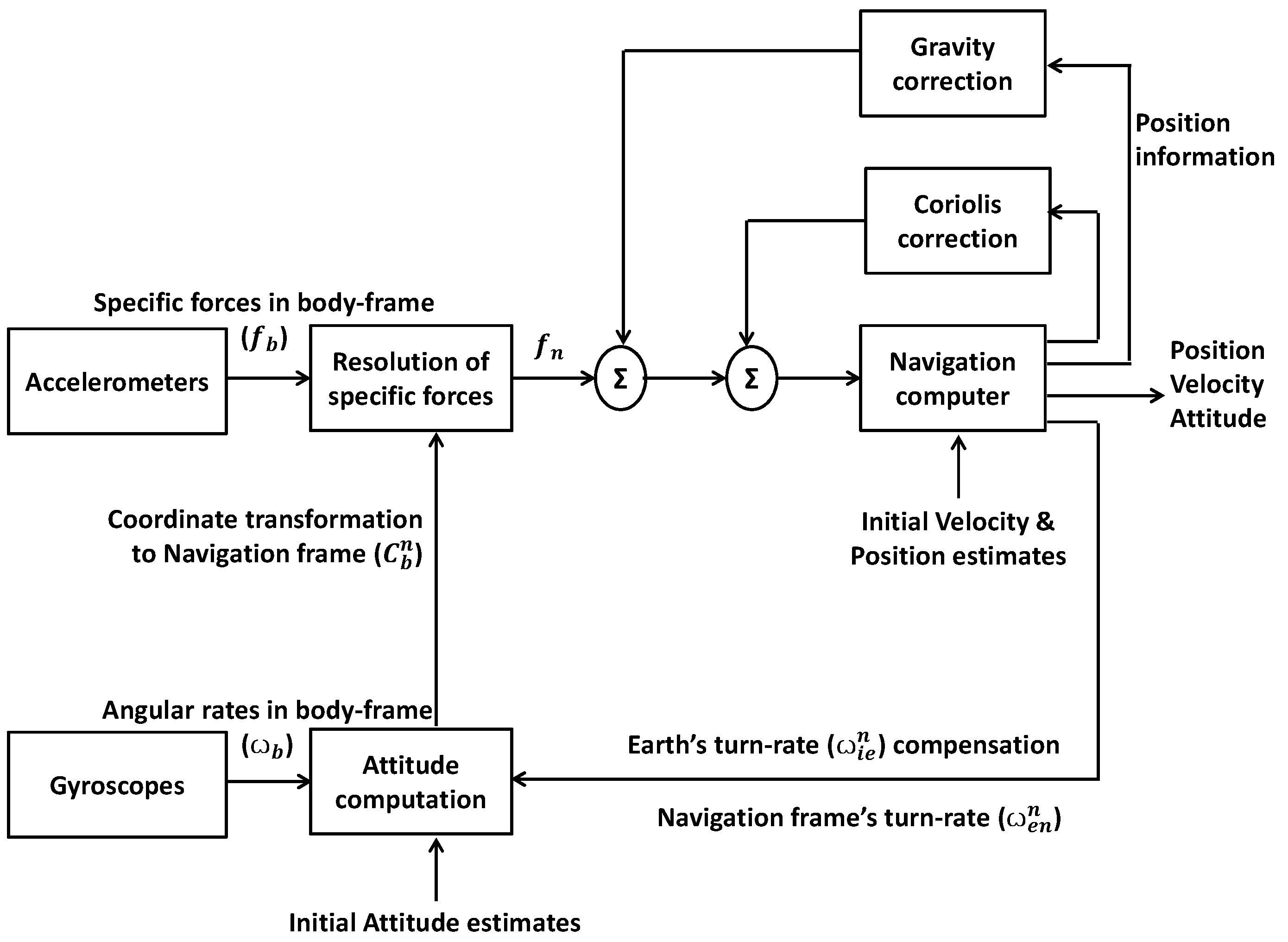
Development of a reliable aided inertial navigation system depends on selecting an appropriate estimation method. The quality of parameter estimates depends chiefly on the type and accuracy of inertial sensors. Thus, the information from sensors should adequately be formulated with careful consideration of error characteristics in each sensor. Based upon the type of coupling, there are two basic GPS/INS integration modes; namely, loose and tight coupling modes [18]. The loosely coupled integration is the simplest and most robust technique of coupling. Navigation solutions are generated by both the INS and the GPS receiver, independently. A third navigation solution is then derived by using an estimator to merge the information provided by the two independent solutions. The Kalman filter including its derivatives is the most widely used filter to realize this fusion [19,20,21]. The fusion Kalman filter calculates error estimates between the two solutions, which are fed back to provide corrected attitude, velocity and position. The robustness of the loosely coupled scheme is due to the fact that if one system fails, the other sensor can still provide navigation, although with reduced accuracy. This research work utilizes the loose coupling strategy for INS-GPS fusion due to its simplicity, robustness, and lesser computational load.
3.1. Conventional Kalman Filter
The Kalman filter is a mathematical estimator used for predicting a system’s behavior from noisy observations. It is a recursive algorithm which uses a series of steps, involving prediction and updating, to obtain an optimal minimum variance estimate of a system or state vector. It is commonly used for estimation in the field of navigation, particularly for autonomous applications [22,23]. It combines noisy sensor outputs (such as those from GPS, accelerometers, and gyroscopes measurements) and estimates the dynamic state of a system (which may include a vehicle’s attitude, acceleration, velocity, position, etc.). For a discrete-time system, the Kalman filter algorithm is given by the following expressions:
Prediction step:
Measurement update step:
where is the state transition matrix; and represent the corrected(or a posteriori) value and the predicted (or a priori) value of the estimated state vector x, respectively; and are the a posteriori and a priori state covariance matrices of order , respectively, at time ; and the matrix of order is the Kalman gain. The term is called the residual or measurement innovation, and is the measurements matrix of order . The matrices Q (of order ) and R (of order ) represent the system and measurement noise covariances, respectively. Assuming that system noise () and measurement noise () are uncorrelated and have characteristics of white noise, we can write the mean matrices as:
And covariance matrices can be written as:
3.2. Adaptive Kalman Filtering
Due to its reliance on a priori information (of dynamic model and noise parameters), the Kalman filter may suffer from degradation or even divergence in situations where this a priori information is time-varying (or unknown) [24]. The matrix R usually contains information provided in a sensor’s data sheet, while the matrix Q is attained analytically. Thus, any errors in Q and/or R may lead to sub-optimal estimation. Although usually taken as constants, Q and R for most practical situations must be adjusted to incorporate time-varying states and sensor inaccuracies which also vary under different dynamic conditions [25,26]. Similarly, in situations where system states are changing abruptly, robustness of the filter also becomes very critical, so that the filter can keep up with sharp changes in observations/measurements. This is achieved by adjusting Kalman gain K, or process covariance matrix P [27]. In order to achieve strong convergence, filter accuracy may have to be suppressed in such cases. This type of filtering is known as adaptive Kalman filtering
3.2.1. Sage-Husa Adaptive Kalman Filter
The Sage-Husa Adaptive Kalman filter [28] is based on a maximum a priori estimation technique. Since the old measurements can influence the estimation process, the filter performance can be optimized by utilizing a finite set of recent measurements. This is achieved by assigning weights to Q and R matrices, which causes the filter to adjust the gain K adaptively. So, in situations where noise statistics vary with time, increasing the weights of latest innovations will lead to enhanced estimation accuracy. For systems with time varying noise characteristics, we can write the mean matrices as
Filtering functions for Sage-Husa–Kalman filter are:
Prediction step:
Measurement update step:
where
The parameter d is known as the attenuation factor, given by
where b is called the forgetting factor. Generally, b is selected using trial and error method but a value between 0.95 and 0.99 has been found to work well [29] to converge the filter to optimal Q and R.
3.2.2. Strong Tracking Robust Kalman Filter
When dealing with inaccurate linear or non-linear dynamic system models, or in situations where state changes are more sudden, the strong tracking filter may provide another effective method for adaptive state estimation [27]. Although lacking in extensive theoretical analysis, the filter has widely been used in practical applications. It makes use of a time varying fading factor which is computed from the most recent measurement innovation, and dynamically corrects the error covariance for state prediction, providing strong tracking of a maneuvering target with abrupt state changes.
The strong tracking Kalman filter algorithm updates the system covariance matrix P by suppressing the filter accuracy, but making it more robust for real time situations, as generalized below:
where the parameter is called the fading factor and is calculated upon the arrival of new measurements, as proposed in [30].
where
and is defined as
and is the measurement innovation given by
The value of parameter is generally taken to be 0.95–0.99. The filter is active only when the system is experiencing abrupt state change (); that is, when
4. Proposed Scheme
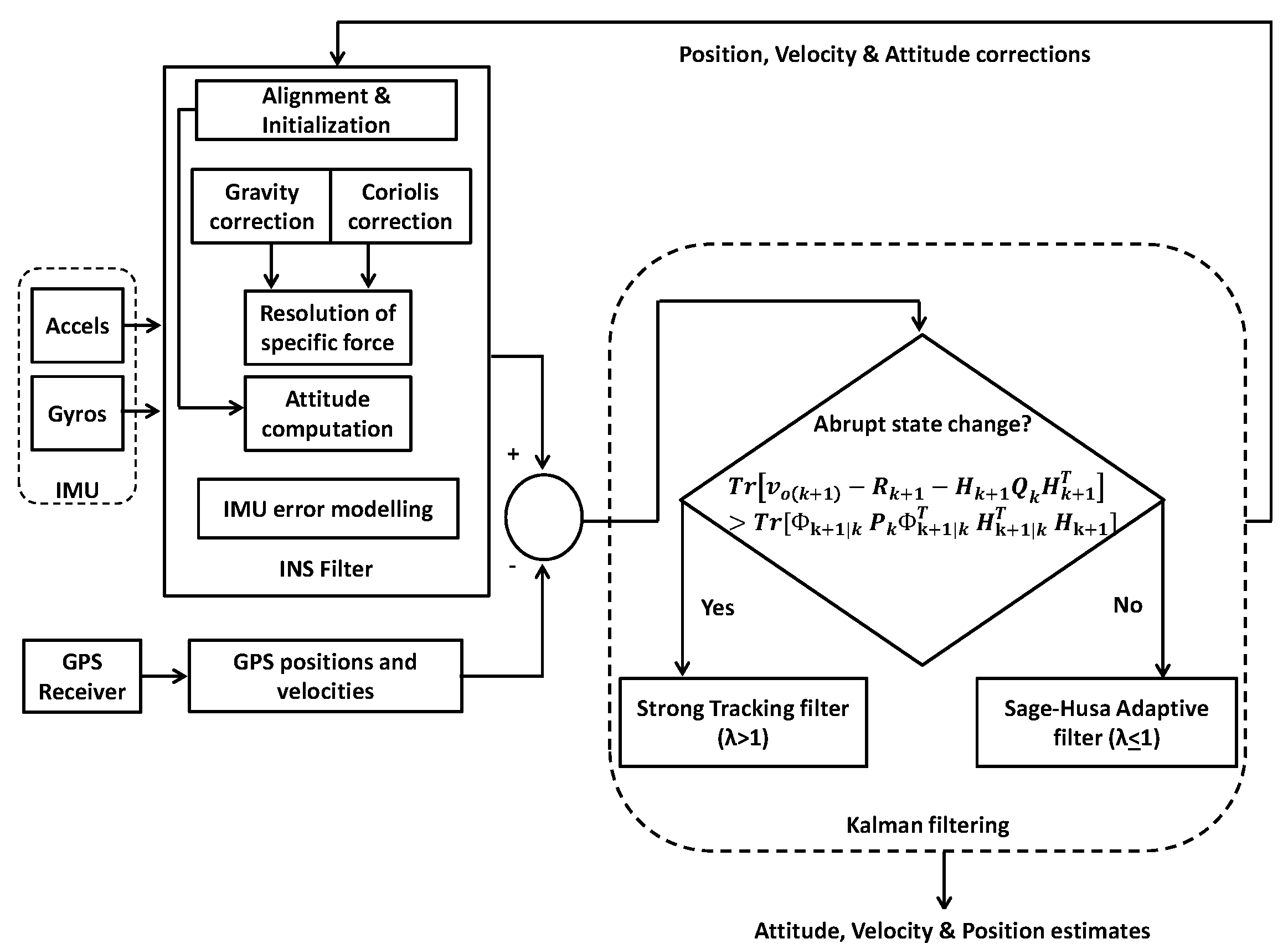
A hybrid filter based on Sage-Husa and strong tracking Kalman filters is presented which offers balance between accuracy and robustness in practical real-time situations where variation in noise statistics is also accompanied by sudden changes in system states. When state change is not abrupt (), the filter will prioritize estimation by Sage-Husa algorithm; otherwise, when , estimation will be carried out through strong tracking filter. The flow diagram demonstrates the filter operation. The filter has been implemented using a loosely coupled scheme due to its simplicity and robustness. The proposed algorithm is depicted in Figure 2.
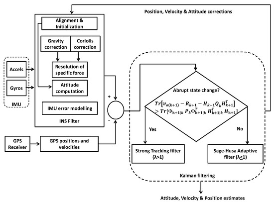
Figure 2.
Proposed scheme.
Mathematical Model
In state-space representation for a linear dynamic system, a system of n-order differential equations is transformed into a set of n-coupled, first-order differential equations. Similarly, for the case of INS-GPS integration, the differential equations representing INS errors can be expressed in a state-space form, which will then be used as system model for Kalman filter. The state-space model consists of two equations; i.e., a dynamic equation and a measurement equation, which can be written respectively as:
where x is state vector of order , F is called system dynamic matrix with order ; w, an vector, represents the system noise; z and v are called the observation vector and the measurement noise vector, respectively, both of order . H is the measurement matrix of order , with m measurements and n states. The above equations can be written in discrete form as:
where is the state vector of order at time ; is the state transition matrix at time ; is the system noise of order ; is the observation vector of order ; is the measurements matrix of order ; and is the measurement noise vector at time . For a discrete-time system, the state transition matrix can be written as:
Taylor series expansion of this equation over a small time interval yields the following expression (ignoring the higher terms):
where I is the identity matrix. The system matrix F is a matrix formed by incorporating the attitude, position and velocity error models of the inertial sensors, which are explained by Titterton in [31]. The system matrix F is given by
where through are all matrices given as
where , , and are the north, east, and down components of specific force, whereas, , , and are the north, east, and down components of vehicle’s velocity, respectively. /hr represents the Earth’s angular speed. and , where and are known as Earth’s meridian radius of curvature and transverse radius of curvature, respectively, when an ellipsoidal model is considered for Earth. , , and represent sin, cos, and tan of the vehicle’s latitude (L), respectively.
where e is the eccentricity of the Earth, with a constant value of , and is known as the equatorial radius of the earth, with value m. The state vector x is given by
where , , and are the errors in roll, pitch, and yaw; , , and are the errors in north, east, and down velocities; and , , and are the errors in latitude, longitude, and altitude, respectively.
The system noise matrix Q consists of variance errors in its principal diagonal and is formed directly from the IMU sensor data sheet, whereas the uncertainties in the GPS measurements are used to derive the measurement noise covariance matrix R.
The difference between GPS and IMU velocity and position measurements forms the measurement vector z.
The latitude and longitude measurements are in radians with very small values, which can make the measurement matrix H singular. This can cause numerical instabilities in Kalman gain K calculation. So the measurement vector can be modified as:
The measurement matrix (H) is written as:
All navigation calculations are being carried out in NED frame of reference.
5. Simulation, Data Collection and Results
The field test drive for data collection each lasting for fifteen minutes was carried out or Murree road (34.156024 N, 73.222560 E), Abbottabad city, Pakistan in January 2019. A total of twenty GPS and IMU measurement data sets were gathered over a period of three days. Two of the data sets were discarded due to erroneous data as a result of a hardware malfunction. Due to mountainous terrain of the city, satellite coverage was moderate and the average number of satellites available was equal to six. In order to avoid any timing errors between the GPS and IMU data, software written in MATLAB was used to time stamp the MEMS IMU data.
The YH-7000 commercial grade MEMS IMU was used for inertial measurements, which include angular rates and specific force data provided by three dimensional gyros and accelerometers. IMU data was obtained at 200 Hz. Simulations have been carried out on real vehicle test drive data in MATLAB R2014A platform (3.1 GHz, Intel, Core i5 CPU). In order to better visualize the filter’s performance for highly dynamic systems, Gaussian noise was introduced to the measurements during the interval between 300 s and 500 s. The actual GPS data was used to compare the estimation results. A total of 250 Monte Carlo simulations were carried out to omit any bias introduced by adding the noise.
Novatel’s OEMV series GPS receiver was used to obtain raw data which was converted to position and velocity measurements using the on-board software at 1 Hz. The GPS measurements included vehicle’s position in terms of latitude, longitude, and altitude, and vehicle’s velocity in terms of north, east and down velocities. Typical error of commercial GPS data is about 30 m in latitude and longitude, while error in altitude is about times greater than latitude/longitude error. The YH-7000 commercial grade MEMS IMU Sensor specifications are given in Table 1:

Table 1.
IMU Sensor specifications.
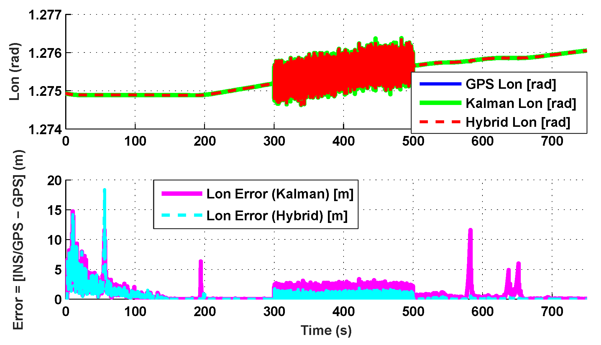
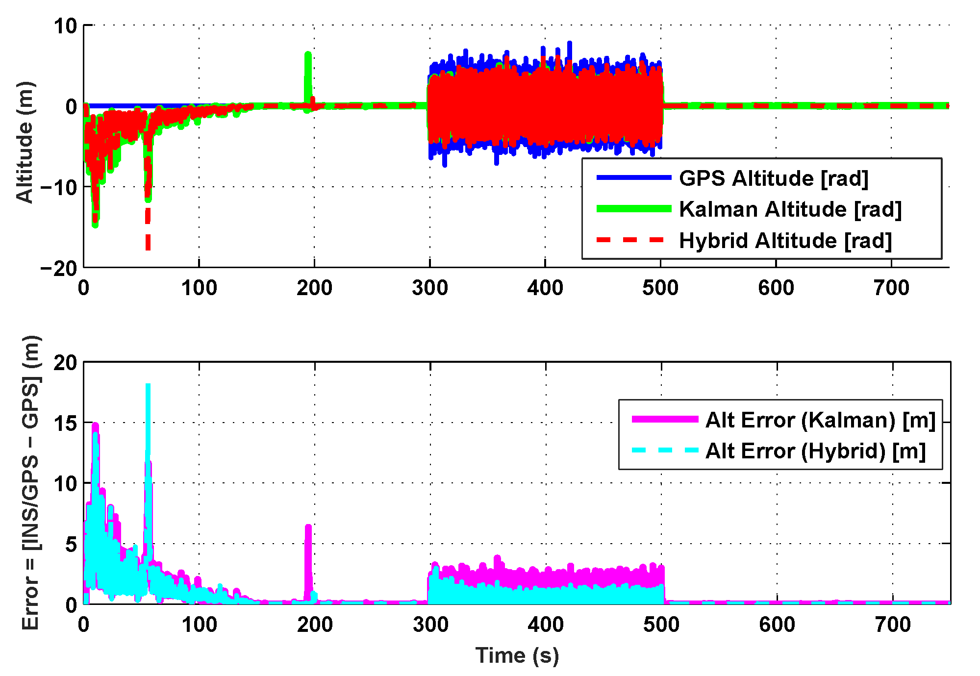
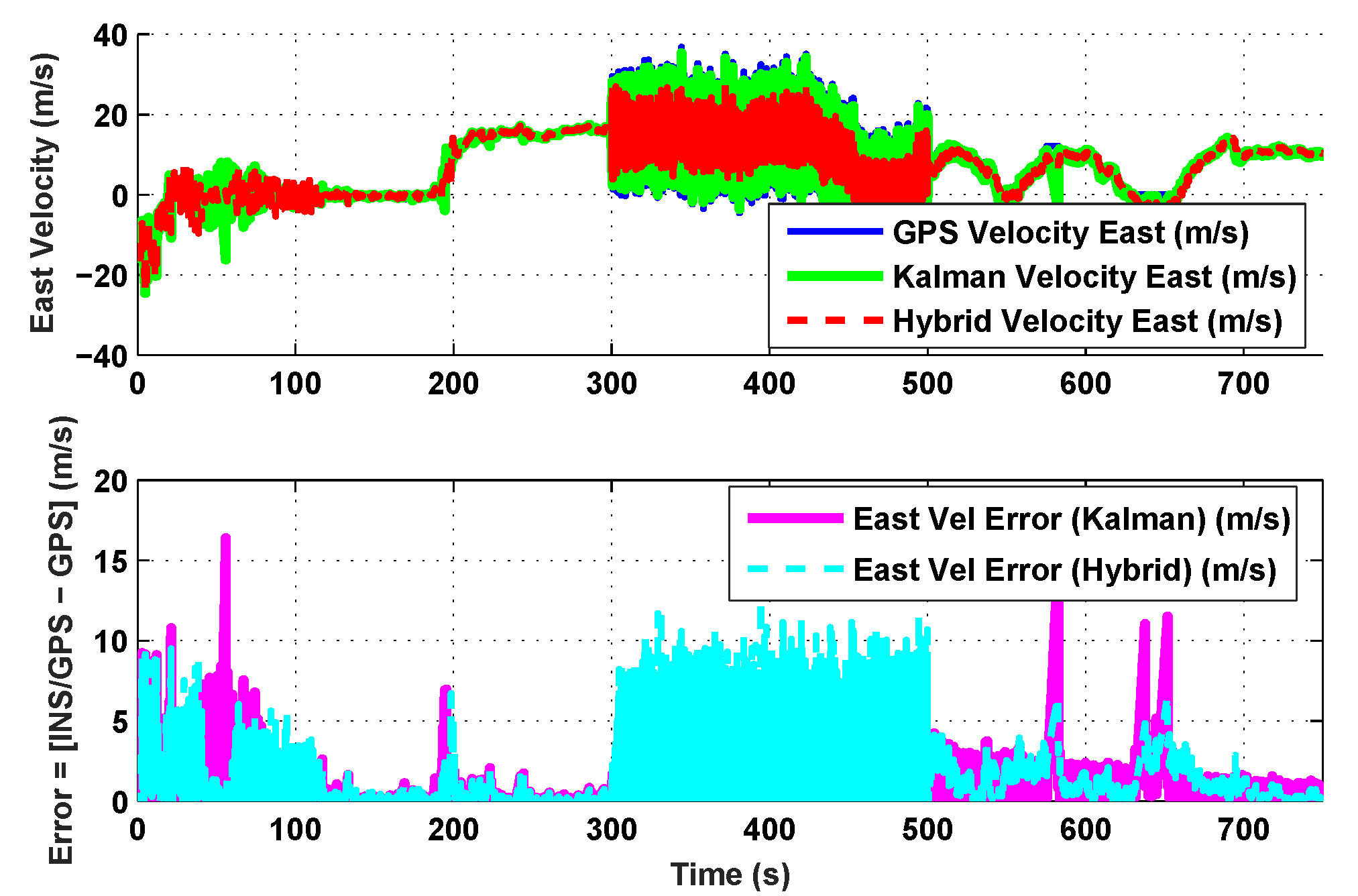
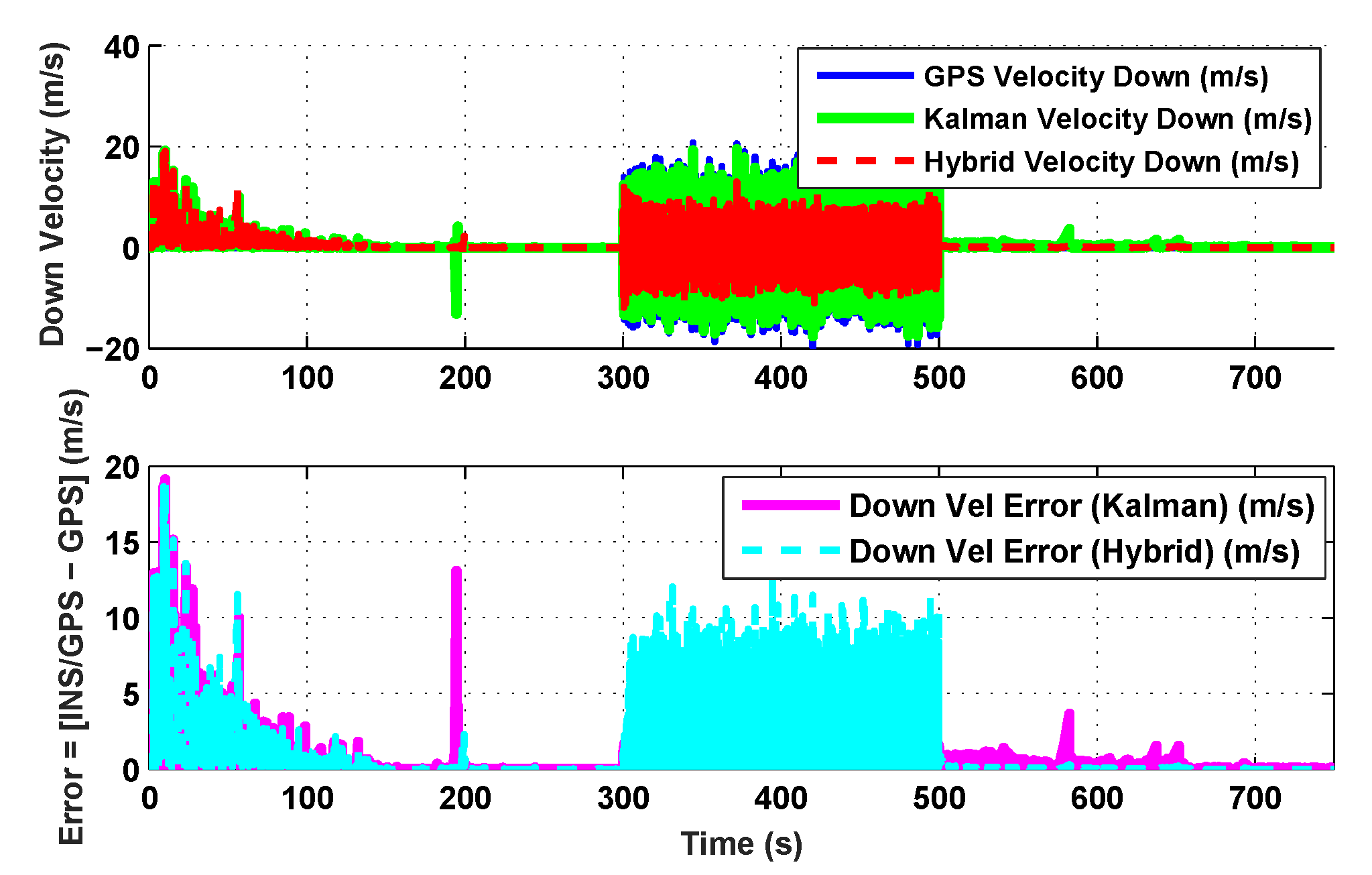
The results for the conventional linear Kalman filter and the hybrid adaptive Kalman filter for INS-GPS integrated navigation are now compared, as shown in the following simulation results with actual sensor data. Vehicle position in terms of latitude, longitude, and altitude is shown first in Figure 3, Figure 4 and Figure 5, whereas vehicle’s velocity in terms of north, east, and down components is shown in Figure 6, Figure 7 and Figure 8, respectively.
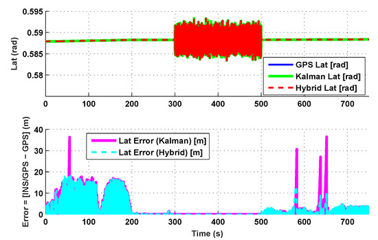
Figure 3.
Latitude comparison.

Figure 4.
Longitude comparison.

Figure 5.
Altitude comparison.
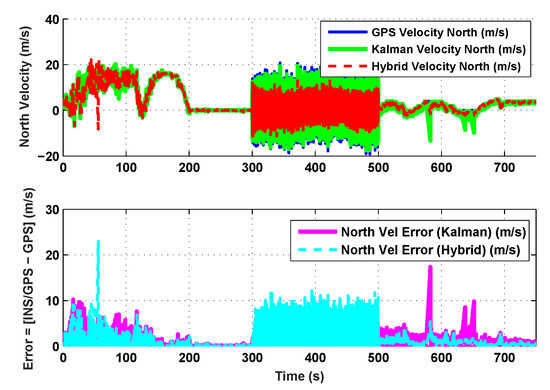
Figure 6.
North velocity comparison.
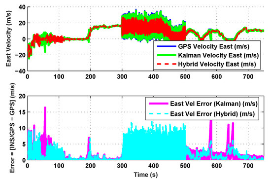
Figure 7.
East velocity comparison.

Figure 8.
Down velocity comparison.
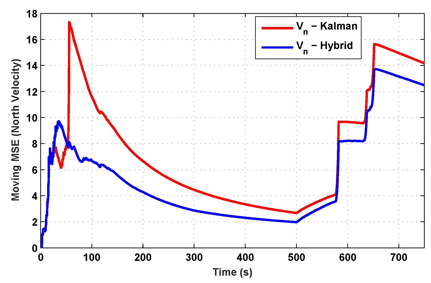
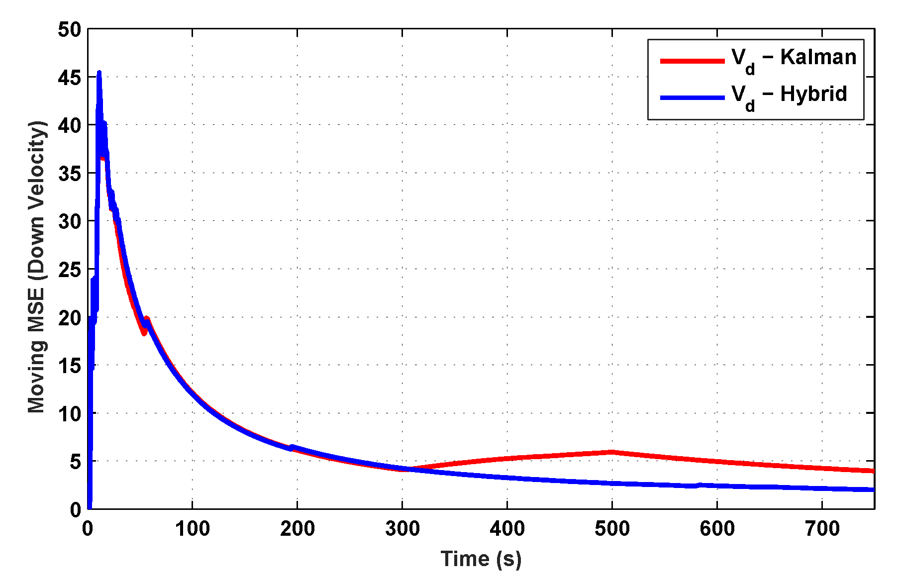
The proposed hybrid filter produces better estimates for vehicle’s position and velocity. Superior performance of the hybrid filter is more evident during the interval between 300 s and 500 s, when random noise was added to the actual sensor measurements. It converges more rapidly compared to the conventional Kalman filter. Similarly, when there is abrupt change in vehicle’s latitude and longitude measurements (near time = 650 s), the hybrid adaptive filter clearly excels at convergence (Figure 3 and Figure 4). This behavior is more pronounced for vehicle’s velocity estimation, which is understandable, given the fact that measurements have been taken for a ground vehicle, which generally experiences more abrupt changes in its velocity/acceleration rather than its position. Figure 6 and Figure 7 clearly show this trend for vehicle’s north and east velocity components.
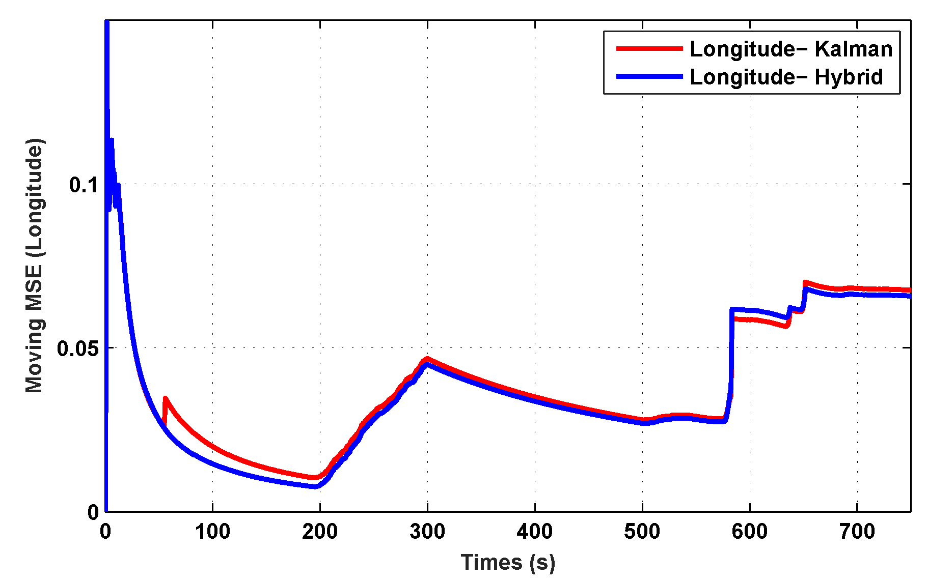
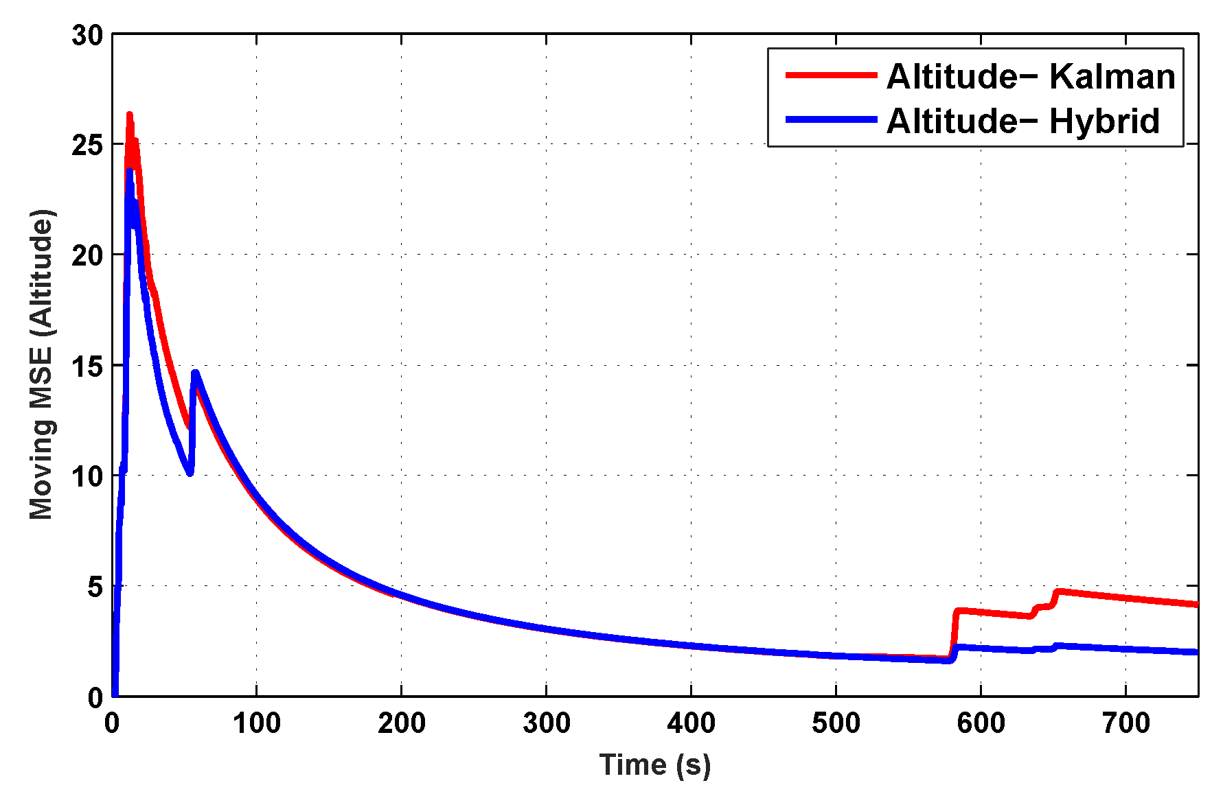
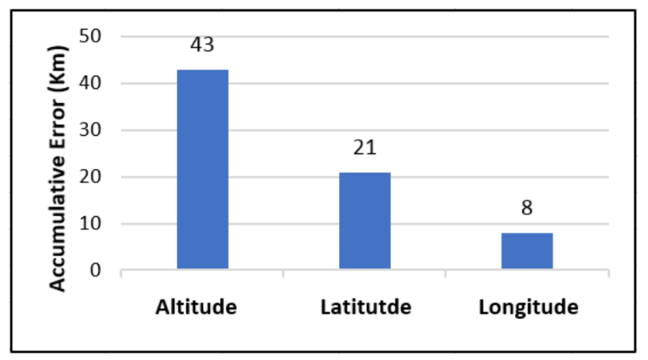
The position and velocity estimation curves for both the linear Kalman filter and the hybrid adaptive Kalman filter appear to be close and the two filters generate almost similar results. However, the hybrid filter, in effect, performs better, which can be seen from the moving mean square error (MMSE) plots of vehicle’s position and velocity (Figure 9, Figure 10, Figure 11, Figure 12, Figure 13, Figure 14 and Figure 15). Overall improvements made by the hybrid filter in vehicle’s position and velocity estimates are also shown by the accumulative error plots of vehicle’s position and velocity in Figure 15 and Figure 16.
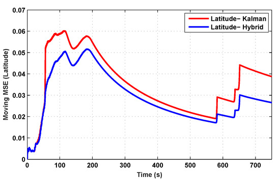
Figure 9.
Moving mean square error (MMSE) comparison in latitude.
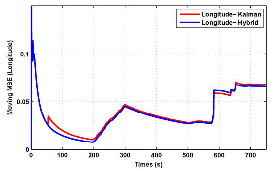
Figure 10.
MMSE comparison in longitude.
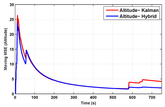
Figure 11.
MMSE comparison in altitude.

Figure 12.
MMSE comparison in northward velocity.
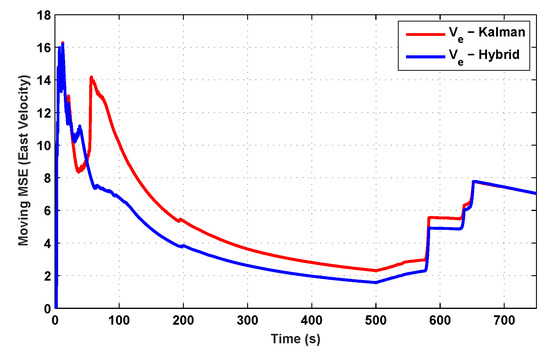
Figure 13.
MMSE comparison in eastward velocity.
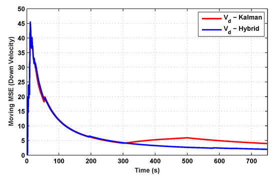
Figure 14.
MMSE comparison in downward velocity.
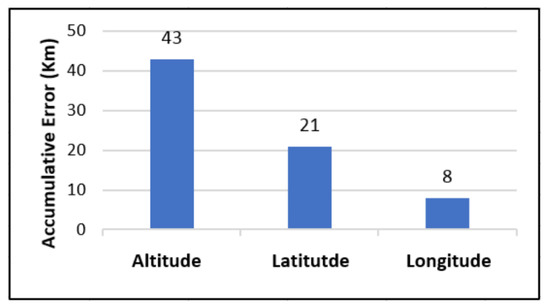
Figure 15.
Difference between errors in position: proposed versus Kalman.
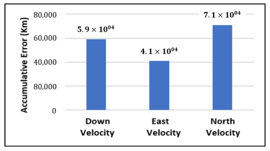
Figure 16.
Difference between errors in velocity: proposed versus Kalman.
The moving mean square error (MMSE) plots provided in Figure 9, Figure 10, Figure 11, Figure 12, Figure 13, Figure 14 and Figure 15 offer a better insight into the performance of proposed hybrid adaptive filter compared to conventional Kalman filter. These curves clearly illustrate superior estimation accuracy of the proposed filter scheme. A quantitative measure of the filter’s accuracy has also been provided in terms of accumulative error plots (Figure 15 and Figure 16), which show overall improvements made by the proposed hybrid scheme in vehicle’s position and velocity estimates.
These results prove the efficiency of the proposed scheme for parameter estimation in navigation, especially for the case when measurements contain large uncertainties/errors, or when states are changing more abruptly, such as the vehicle’s velocity.
Switching decision between the Sage-Husa filter and the robust tracking filter is made based on the check provided in Equation (45). When an anomaly in the measurements is detected, like a large error, or abrupt state change, the condition in Equation (45) is satisfied, and the filter switches to robust mode where more weight is assigned to latest measurements, thus, providing strong tracking of the target.
6. Conclusions
A novel algorithm based on a hybrid of the Sage-Husa filter and the strong tracking filter using a loosely coupled scheme is proposed for GPS-INS integration. The proposed algorithm has generated superior navigation for a vehicle’s position and velocity estimates. The algorithm offers a balance between accuracy and strong convergence for optimum estimation for highly dynamic systems. It inherently performs much better when implemented for more dynamic systems, as proven by the results. The same hybrid filter will, thus, produce even better navigation estimates for target tracking applications or in case of aerial vehicles, where a conventional Kalman filter will certainly lag behind due to its reliance on a priori information, and consequently, its inability to keep track of sudden changes in system states. The hybrid filter based on Sage-Husa–Kalman filter and strong tracking Kalman filter can, thus, be acknowledged as an optimal filter when compared to the conventional Kalman filter.
Author Contributions
Data curation, S.M.; formal analysis, U.K., M.B.Q., and M.U.S.K.; funding acquisition, M.U.S.K. and R.N.; investigation, H.A., I.U., and M.B.Q.; methodology, S.M. and N.M.; Project administration, R.N.; Software, H.A.; supervision, I.U.; validation, H.A. and R.N.; visualization, N.M.; writing—original draft, H.A. and I.U.; writing—review and editing, U.K.
Funding
This research received no external funding.
Conflicts of Interest
The authors declare no conflict of interest.
References
- Choi, E.; Chang, S. A consumer tracking estimator for vehicles in GPS-free environments. IEEE Trans. Consum. Electron. 2017, 63, 450–458. [Google Scholar] [CrossRef]
- Bevly, D.M.; Parkinson, B. Cascaded Kalman filters for accurate estimation of multiple biases, dead-reckoning navigation, and full state feedback control of ground vehicles. IEEE Trans. Control Syst. Technol. 2007, 15, 199–208. [Google Scholar] [CrossRef]
- Kirkko-Jaakkola, M.; Collin, J.; Ta, J. Bias prediction for MEMS gyroscopes. IEEE Sens. J. 2012, 12, 2157–2163. [Google Scholar] [CrossRef]
- Savage, P. Strapdown Analytics, Part 1; Strapdown: Maple Plain, MN, USA, 2007. [Google Scholar]
- Perera, L.D.; Wijesoma, W.S.; Adams, M.D. The estimation theoretic sensor bias correction problem in map aided localization. Int. J. Robot. Res. 2006, 25, 645–667. [Google Scholar] [CrossRef]
- Atia, M.M.; Liu, S.; Nematallah, H.; Karamat, T.B.; Noureldin, A. Integrated indoor navigation system for ground vehicles with automatic 3-D alignment and position initialization. IEEE Trans. Veh. Technol. 2006, 64, 1279–1292. [Google Scholar] [CrossRef]
- Salmon, D.C.; Bevly, D.M. An Exploration of Low-cost Sensor and Vehicle Model Solutions for Ground Vehicle Navigation. In Proceedings of the IEEE/ION Position, Location and Navigation Symposium-PLANS 2014, Monterey, CA, USA, 5–8 May 2014. [Google Scholar]
- Tahir, Z.; Qureshi, A.; Ayaz, Y.; Nawaz, R. Potentially guided bidirectionalized RRT* for fast optimal path planning in cluttered environments. Robot. Auton. Syst. 2018, 108, 13–27. [Google Scholar] [CrossRef]
- Sukkarieh, S.; Nebot, E.M.; Durrant-Whyte, H.F. Achieving integrity in an INS/GPS navigation loop for autonomous land vehicle applications. In Proceedings of the 1998 IEEE International Conference on Robotics and Automation, Leuven, Belgium, 20–20 May 1998; Volume 4, pp. 3437–3442. [Google Scholar] [CrossRef]
- Rose, C.; Britt, J.; Allen, J.; Bevly, D. An Integrated Vehicle Navigation System Utilizing Lane-detection and Lateral Position Estimation Systems in Difficult Environments for GPS. IEEE Trans. Intell. Transp. Syst. 2014, 15, 2615–2629. [Google Scholar] [CrossRef]
- Qadir, H.; Khalid, O.; Khan, M.; Khan, A.; Nawaz, R. An Optimal Ride Sharing Recommendation Framework for Carpooling Services. IEEE Access 2018, 6, 62296–62313. [Google Scholar] [CrossRef]
- Ayyaz, S.; Qamar, U.; Nawaz, R. HCF-CRS: A Hybrid Content based Fuzzy Conformal Recommender System for providing recommendations with confidence. PLoS ONE 2018, 13, e0204849. [Google Scholar] [CrossRef]
- Godha, S.; Cannon, M.E. Integration of DGPS with a low cost MEMS-based inertial measurement unit (IMU) for land vehicle navigation application. In Proceedings of the 18th International Technical Meeting of the Satellite Division of the Institute of Navigation, Long Beach, CA, USA, 13–16 September 2005; pp. 333–345. [Google Scholar]
- Zhao, S.; Chen, Y.; Farrell, J.A. High-precision Vehicle Navigation in Urban Environments Using an MEM’s IMU and Single-frequency GPS Receiver. IEEE Trans. Intell. Transp. Syst. 2016, 17, 2854–2867. [Google Scholar] [CrossRef]
- Schmidt, G.T. Navigation Sensors and Systems in GNSS Degraded and Denied Environments. Chin. J. Aeronaut. 2015, 28, 1–10. [Google Scholar] [CrossRef]
- Grewal, M.S.; Andrews, A.P.; Bartone, C.G. Global Navigation Satellite Systems, Inertial Navigation, and Integration, 3rd ed.; Wiley-Interscience: New York, NY, USA, 2013. [Google Scholar]
- Nisar, S.; Ullah, I. Non-linear filtering techniques for high precision GPS applications. In Proceedings of the 2017 International Conference on Communication, Computing and Digital Systems, Islamabad, Pakistan, 8–9 March 2017; pp. 276–280. [Google Scholar] [CrossRef]
- Chen, Z.; Qu, Y.; Ling, X.; Li, Y.; Jiao, H.; Liu, Y. Study on GPS/INS loose and tight coupling. In Proceedings of the 7th International Conference on Intelligent Human-Machine Systems and Cybernetics, Jiangyin, China, 26–27 August 2015. [Google Scholar]
- El-Diasty, M.; Pagiatakis, S. An efficient INS/GPS impulse response model for bridging GPS outages. In Proceedings of the 2009 IEEE Toronto International Conference Science and Technology for Humanity (TIC-STH), Toronto, ON, Canada, 26–27 September 2009. [Google Scholar]
- Crassidis, J.L. Sigma-point Kalman filtering for integrated GPS and inertial navigation. IEEE Trans. Aerosp. Electron. Syst. 2006, 42, 750–756. [Google Scholar] [CrossRef]
- Gupta, M. The Strong Tracking Augmented Kalman Filter for Satellite Attitude Determination. Int. J. Adv. Res. Sci. Eng. 2014, 3, 171–180. [Google Scholar]
- Karlgaard, C.D.; Shen, H. Desensitised Kalman filtering. IET Radar Sonar Navig. 2013, 7, 2–9. [Google Scholar] [CrossRef]
- Zanetti, R.; Bishop, R.H. Kalman filters with uncompensated biases. J. Guid. Control Dyn. 2012, 35, 327–335. [Google Scholar] [CrossRef]
- Zheng, B.; Fu, P.; Li, B.; Yuan, X. A robust adaptive unscented Kalman filter for nonlinear estimation with uncertain noise covariance. Sensors 2018, 18, 808. [Google Scholar] [CrossRef]
- Ding, W.; Wang, J.; Rizos, C. Improving adaptive Kalman estimaion in GPS/INS integration. J. Navig. 2007, 60, 517–529. [Google Scholar] [CrossRef]
- Jaradat, M.A.K.; Abdel-Hafez, M.F. Enhanced, Delay Dependent, Intelligent Fusion for INS/GPS Navigation System. IEEE Sens. J. 2014, 14, 1545–1554. [Google Scholar] [CrossRef]
- Ge, Q.; Shao, T.; Wen, C.; Sun, R. Analysis on strong tracking filtering for linear dynamic systems. Math. Probl. Eng. 2015, 2015, 648125. [Google Scholar] [CrossRef]
- Sage, A.P.; Husa, G.W. Adaptive filtering with unknown prior statistics. IEEE Trans. Autom. Control 1969, 7, 760–769. [Google Scholar]
- Sun, F.; Zhang, H. Application of a new adaptive Kalman filtering algorithm in initial alignment of INS. In Proceedings of the 2011 IEEE International Conference on Mechatronics and Automation, Beijing, China, 7–10 August 2011. [Google Scholar]
- Zhou, D.H.; Xi, Y.G.; Zhang, Z.J. A suboptimal multiple fading extended Kalman filter. Chin. J. Autom. 1991, 4, 145–152. [Google Scholar]
- Titterton, D.; Weston, J. Strapdown Inertial Navigation Technology, 2nd ed.; The Institution of Engineering and Technology: London, UK, 2005. [Google Scholar]
© 2019 by the authors. Licensee MDPI, Basel, Switzerland. This article is an open access article distributed under the terms and conditions of the Creative Commons Attribution (CC BY) license (http://creativecommons.org/licenses/by/4.0/).


