Article

A Novel Surface Descriptor for Automated 3-D Object Recognition and Localization

by
Liang-Chia Chen
1,* and
Thanh-Hung Nguyen
2
1
Department of Mechanical Engineering, National Taiwan University, Taipei 10617, Taiwan
2
Department of Mechatronics, School of Mechanical Engineering, Hanoi University of Science and Technology, 1 Dai Co Viet Road, Hanoi 112400, Vietnam
*
Author to whom correspondence should be addressed.
Sensors 2019, 19(4), 764; https://doi.org/10.3390/s19040764
Submission received: 27 December 2018 / Revised: 3 February 2019 / Accepted: 10 February 2019 / Published: 13 February 2019
(This article belongs to the Special Issue Sensor Applications for Smart Manufacturing Technology and Systems)

Abstract

:
This paper presents a novel approach to the automated recognition and localization of 3-D objects. The proposed approach uses 3-D object segmentation to segment randomly stacked objects in an unstructured point cloud. Each segmented object is then represented by a regional area-based descriptor, which measures the distribution of surface area in the oriented bounding box (OBB) of the segmented object. By comparing the estimated descriptor with the template descriptors stored in the database, the object can be recognized. With this approach, the detected object can be matched with the model using the iterative closest point (ICP) algorithm to detect its 3-D location and orientation. Experiments were performed to verify the feasibility and effectiveness of the approach. With the measured point clouds having a spatial resolution of 1.05 mm, the proposed method can achieve both a mean deviation and standard deviation below half of the spatial resolution.

Graphical Abstract

1. Introduction

Nowadays, both 2-D and 3-D machine vision systems are widely integrated with robot manipulators to enhance the flexibility and versatility of modern manufacturing systems. These intelligent integrated systems can accelerate manufacturing and produce efficiently customized products to enhance competitiveness. 2-D machine vision systems [1,2,3,4] are still used in most integrated systems due to their high accuracy and low cost. However, the operation accuracy in these systems is limited by the viewing angle of optical sensing and is especially sensitive to the alignment precision of the jig and fixture employed in locating the workpiece. Systems that involve 3-D data processing can overcome the existing difficulties in 2-D digital imaging by relying on both shape and color information of the objects. These systems have recently been integrated with automated machine manipulators for pick and place applications [5,6,7,8,9,10,11].
One of the most important tasks in 3-D data processing is to determine the position and orientation of the target in 3-D space. This task remains challenging in automation because the target can be of any geometric form and its positioning orientation has six degrees of freedom. Thus, it is difficult to detect the target with an unstructured data input, such as range point clouds. In recent years, several attempts have been made to solve this nontrivial problem. According to their characteristics, the proposed strategies can be divided into graph-based, feature-based, and view-based methods.
Graph-based methods extract the geometric properties of a 3-D shape using a graph, which represents the type and spatial relations between shape components [6,7,12]. In these approaches, the topology graph is built using the detected primitive shapes in the scanned scene. The query graph, which represents the structure of the CAD model and is manually defined by the user, is employed to search the target in the topology graph. Fuchs et al. [6] substituted two parallel lines for a pipe. The distance between two lines is the diameter of the pipe. Skotheim et al. [7] defined a car part as a graph containing two vertices and an edge. One vertex represents a reference plane and the other vertex describes a search plane. The edge of the graph is associated with the distance and relative orientation between the centers of the reference and search planes. More generally, Schnabel et al. [12] presented the scanned data with a topology graph, in which the vertices of the graph are the detected shapes (planes, cylinders, spheres, and cones) and the edges of the graph joined the connected shapes. This technique had been integrated with the service robot for bin picking [10]. Graph-based methods are pose-independent and the graph-based structure can be used for partial matching. However, the matching criteria depend on the structure of the 3-D shape and the computation time involved could be extremely high. Moreover, for graph-based methods, the similarity measure is sensitive to changes in topology. These methods are commonly used in applications, in which the form of the target object is composed of a few simple primitive shapes, such as planes, cylinders, spheres, and cones.
Feature-based methods [13,14,15,16,17,18,19] discriminate 3-D objects by measuring and comparing the geometric and topological properties of 3-D shapes. The points that contain sufficient information to distinguish the shape from others are extracted from the scanned data and defined as feature points. The local information around feature points is then employed to build the local 3-D descriptor. The target object is recognized by matching the scene descriptors with model descriptors. Johnson and Hebert [13] presented the spin image, which was created by projecting the 3-D points into 2-D images for object matching. Chen and Bhanu [14] investigated the relation between the shape index (SI) and the dot product of the surface normal to establish a local surface patch descriptor for object recognition. Zaharescu et al. [15] computed the gradient for each feature point and the histogram of the gradient (HOG) both spatially at a coarse level and a fine level to obtain the MeshHOG descriptor for mesh matching. Drost et al. [16] introduced the point pair feature to describe the geometric information, aligning the model point pairs with the scene point pairs for 3-D object recognition. Rusu et al. [17] considered the relationships between the points in the k-neighborhood of the feature point and their estimated surface normals to build the fast point feature histogram (FPFH) descriptor. By encoding the important statistics between the viewpoint and the surface normals on the object into the extended FPFH descriptor to perform the viewpoint feature histogram (VHF), the object and its pose can be simultaneously recognized in the scene point clouds. Salti et al. [18] generated a local histogram according to the distribution of the normal vector at the feature point. These local histograms are then categorized together to form the actual descriptor, which is called the signature of histograms of orientations (SHOT). More recently, geometric information has been used in object recognition [19]. Feature-based maximum-likelihood matching by a simple two-degree-of-freedom analysis of 3D point cloud data demonstrated effect view-based veness in automated object recognition [20]. However, feature-based methods are good when only partial data are available. In general, the descriptors are less discriminative from a global matching point of view. In general, these methods can work best when having geometric details, but are less efficient in comparison to other methods.
View-based methods recognize the target object according to the principle that two 3-D objects are only similar when they look similar from all viewing angles [8,11,21]. In these methods, a real range image acquired from a 3-D scanner can be matched with a set of range images stored in the template database. The database is generally generated from the 3-D model of the object from all possible viewing angles. Liu et al. [8] represented scanned data with a depth-edge map. The database of depth-edge templates is created from a CAD model by detecting the depth discontinuities in the model. Each template is then compared with the depth-edge map to determine the position and location of the target object in the scanned scene. Sansoni et al. [11] separated the scanned data into individual segmented point clouds. Each segmented point cloud is then matched using a commercial software with a set of 3-D templates, which are acquired from different viewpoints of the real object. In the approach proposed by Chen, the segmented object is represented by the curvature-based histogram, which is computed using the shape index value of every point of the segmented object [21]. The target object can be recognized by comparing the computed curvature-based histogram with the template histograms in the database. View-based methods can be applied to almost all kinds of objects. However, the disadvantage is that the comparison of the database and the acquired data is time-consuming.
From the above review, it can be seen that one of the reasons why the 3-D vision system has not been widely used in robotic automation is the long computation time required for practical application. In view of this, a fast and effective method for 3-D object recognition and localization is proposed to deal with the difficulties existing in this task. The main idea of the approach is that two objects are similar if the distributions of their surface areas in their oriented bounding boxes (OBBs) are the same.
In this study, the proposed approach for 3D object recognition and localization can deal with the difficulties existing for practical applications such as robotic automation. The developed method proposes a new index for 3-D object recognition with a good efficiency in operation and robustness to illumination variations. In addition, the key solution can recognize stacked objects with arbitrary orientation. The main idea of the approach starts from the point that two objects are similar if the distributions of their surface areas in their OBBs are the same. The method comprises two main stages. In the first stage, the proposed regional area-based descriptors are computed for implementing the shape-matching algorithm for reliable object recognition. In the second stage, the position and orientation of the target are initially determined by aligning the OBBs and further refinement by the iterative closest point (ICP) algorithm.
The rest of this paper is organized as follows. Section 2 presents the proposed method for object recognition and localization employing regional area-based descriptors. The experimental results and analysis are shown in Section 3. Section 4 discusses the characteristics and limitations of the developed method in detail. Finally, the conclusions and further work are summarized in Section 5.

2. Methodology

Given a point cloud that represents the scene of the randomly stacked objects in an unstructured bin, the task is to recognize and localize the target object in the scene point clouds. To deal with the task, the proposed approach first separates the scene point clouds into individual object point clouds [22]. Each segmented object can be represented by a feature vector, which is computed according to its OBB and object surface area. The feature vector is then matched with the feature vectors kept in the database, which represent the different views of the object model. According to the matching results, the transformation matrix can be initially computed to align the segmented object with the object model. Finally, the 3-D position and orientation of the target object in the scene point clouds can be estimated using the ICP algorithm. The overview and flowchart of the proposed method are shown in Figure 1 and Figure 2, respectively. In addition, the operation procedure of the proposed method is described in Algorithm 1.
Algorithm 1:
Input: Measured point cloud O and model point cloud M.
Output: Position and Orientation of objects.
  • Segmentation: Segment scene point cloud into individual object point clouds (Segmentation) O = {Oj, j = 0, 1, …, n}. (Section 2.1)
  • Compute descriptor of each segmented individual object point cloud FVO = {FVOj, j = 0, 1, …, n} (Section 2.2)
  • 3D Virtual Camera: Extract m point clouds corresponding to m different views of the model point cloud using 3D virtual sensor (result: M = {Mi, i = 0, 1, …, m}) and compute the descriptors (result: FVM = {FVMi, i = 0, 1, …, m}). (Section 2.3)
  • Recognition: Match the descriptors of Oj and M, determine the best matching, and obtain corresponding points of Oj in M, MOj. (Section 2.4.1 and Section 2.4.2)
  • Localization: Align the OBB of the point cloud Oj and OBB of the corresponding point cloud MOj. Obtain the initial transformation matrix, and then apply the Iterative Closest Point (ICP) algorithm for refinement. (Section 2.4.3)

2.1. Object Segmentation

The point cloud data acquired from the 3-D scanner comprises information of one view of different objects in the scene. In order to obtain the segmented point clouds corresponding to one view of an object for a later recognition task, the scene point clouds should be further separated into smaller point clouds. In recent years, many techniques have been developed to obtain the individual parts from the point cloud data. The popular techniques are the region growing method [23,24], k-nearest neighbors clustering algorithm [25,26], and graph theoretic approach [27,28,29].
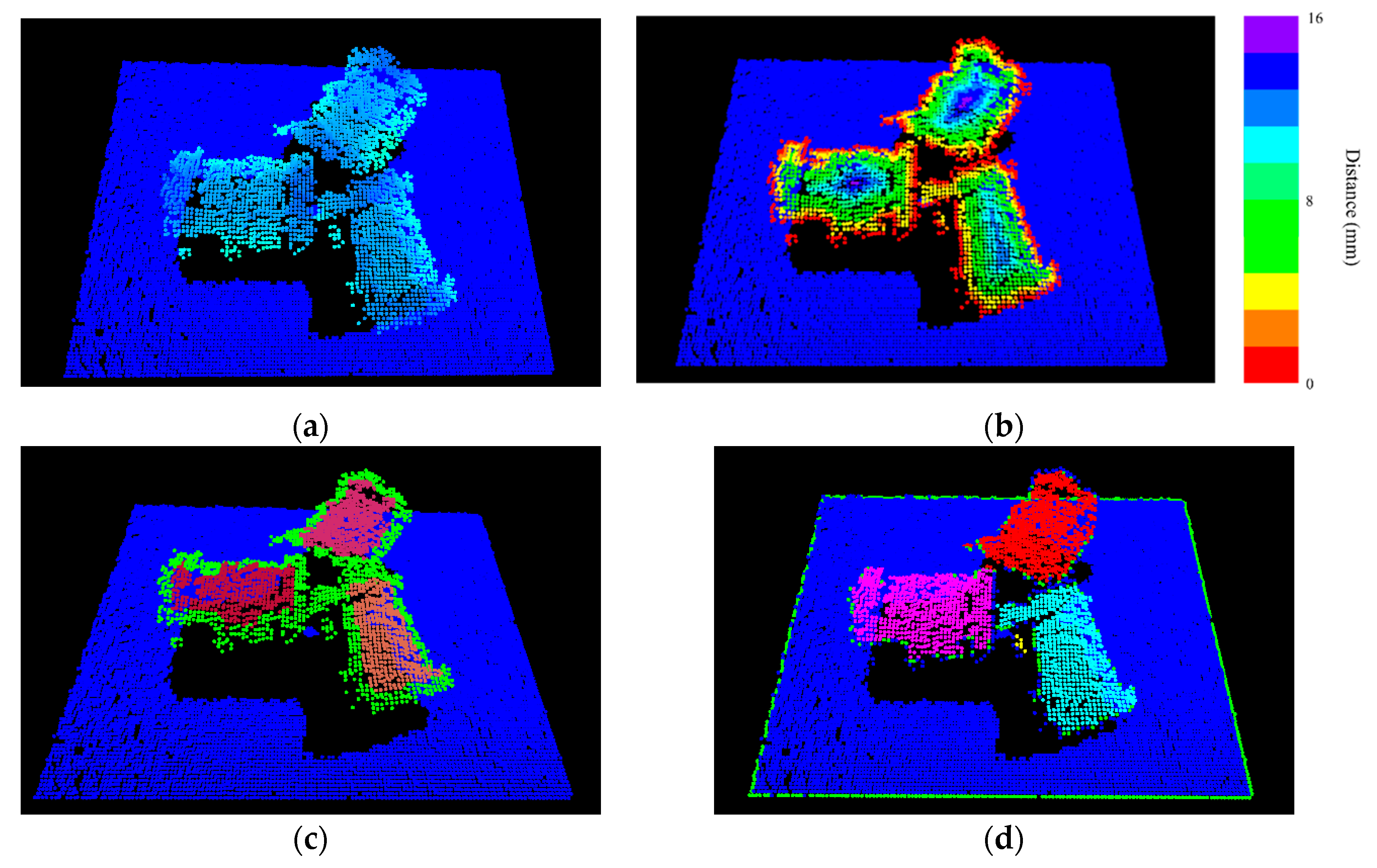
In this study, the developed 3-D object segmentation algorithm for randomly stacked objects [29,30] is employed to obtain the segmented point clouds corresponding to the object in the scene point clouds. The basic idea of the proposed algorithm is that the points located geometrically farther from the surface boundary of the projected object are more likely to belong to the same object than the other points (as shown in Figure 3b). The points far away from the surface boundary can be used as an internal seed marker for object region growth (as illustrated in Figure 3c). With a flooding algorithm, the scene point clouds can be clearly separated into smaller individual object point clouds (see Figure 3d). The general process of the proposed algorithm is presented in Figure 3.

2.2. Regional Area-based Descriptor

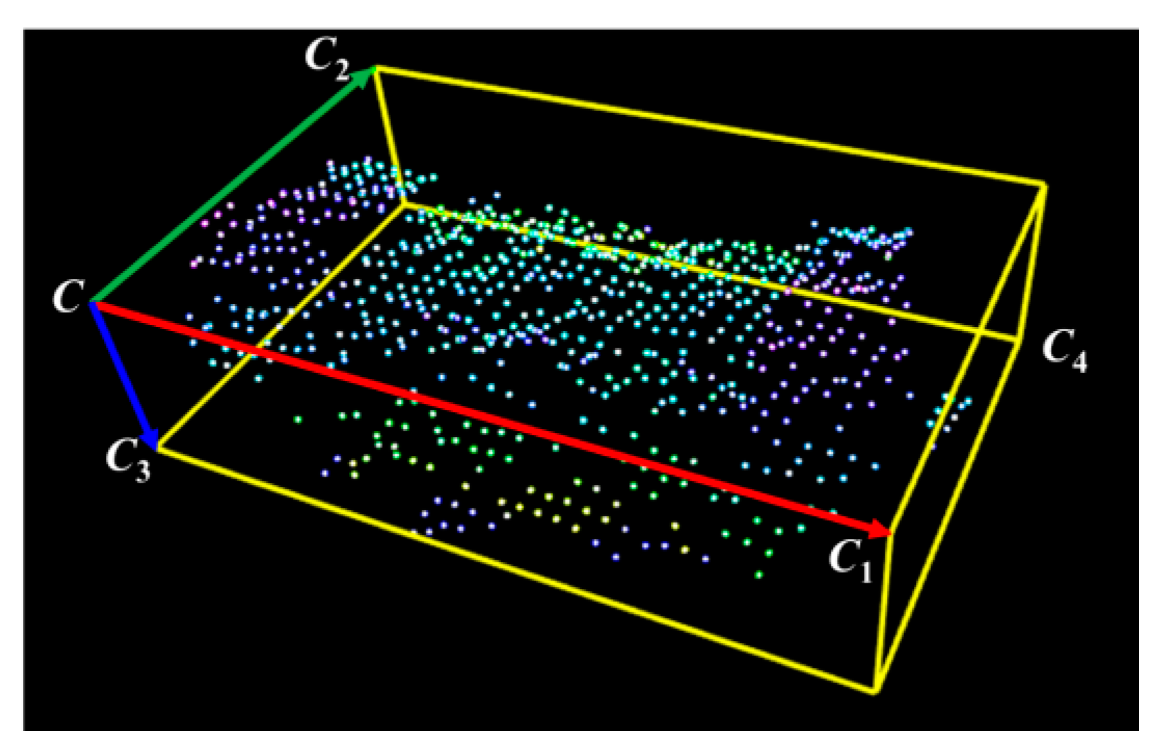
To find the similarity between the point cloud model M and the segmented point cloud O, which is extracted using the object segmentation algorithm, the feature descriptor of the segmented object is compared with the feature descriptors of different views of the model. A feature descriptor is normally defined by two essential elements [30], namely the OBB and surface area of the object. An OBB consists of a corner and three principle vectors (shown in Figure 4). The surface area of the object defines the histogram of all the surface areas within the OBB. In general, the total number of subdivided boxes is k1 × k2 × k3 when the OBB is defined by k1, k2, and k3 (shown in Figure 5). The surface area in each subdivided box (Vijk) is described as Sv, in which v = kk1k2 + jk1 + i. Let S be the total surface area of the segmented object in the OBB and fv equal Sv/S. The feature descriptor can be described as follows:
F V = { C , C C 1 , C C 2 , C C 3 , f 0 , , f v , , f n V } ,
where
  • nV = k1k2k3 − 1;
  • C: corner vector;
  • CC1, CC2, and CC3: principle vectors corresponding to the maximum, middle, and minimum dimensions of the OBB, respectively.
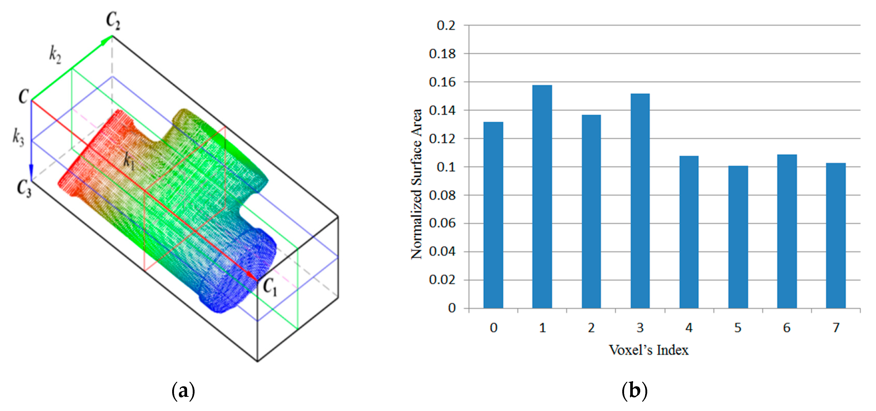
Finally, according to Sv, the regional area-based descriptor can be built as shown in Figure 6. In this example, the OBB of the object point clouds is subdivided into eight sub-boxes. In addition, three parameters k1, k2, and k3 are set to equal 2.
The proposed descriptor utilizes the distribution of the object’s surface area inside the OBB of the object to represent the object in 3D space. The OBB regional area-based descriptor is invariable to arbitrary poses of the objects, because the surface area is an intrinsic property that is completely independent of object positions and orientations in space. Furthermore, the developed approach is robust to numerous variations of surface sampling density and noise generated from the measurement process. In order to match the model point cloud and the segmented point cloud extracted using the object segmentation algorithm, the feature descriptor of the segmented object is compared with the feature descriptors of various views of the model in the database using normalized cross-correlation (NCC).
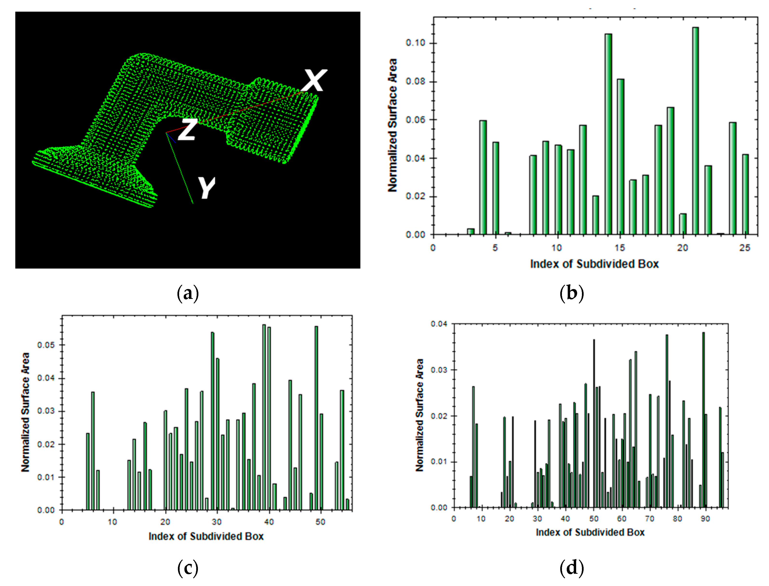
The total number (n) of subdivided boxes in the OBB is an important parameter for computation efficiency. When the OBB contains more subdivided boxes, matching normally takes more time and the matching accuracy is thus increased. To shorten the matching procedure, fewer subdivided boxes are preferable. However, to ensure matching accuracy, the number of subdivided boxes should be adequately set to achieve meaningful matching. Figure 7 illustrates three examples of the regional area-based descriptors of an L-shape object with three different types of segments, in which n (= k1 × k2 × k3) is computed as 5 × 5 × 1, 5 × 4 × 3, and 5 × 5 × 4, respectively, with the running time being 0.15, 0.35, and 0.65 s, respectively.

2.2.1. Estimation of Oriented Bounding Box

The OBB of an object is a rectangular bounding box that covers all object point clouds. The orientation of an OBB can be determined using the covariance matrix [31]. The associated algorithm is described in the following steps:
Calculate the center p ¯ of the point cloud P;
Compute the covariance matrix:
C O V = 1 n i = 1 n ( p i p ¯ ) ( p i p ¯ ) T ;
Extract the eigenvectors {v1, v2, v3} from the covariance matrix;
Determine the dimensions of the object defined in each eigenvector using the distances between the nearest and farthest projected points.
The corner C(xC, yC, zC) farthest from the center p ¯ will be chosen from eight corners of the OBB. Then, the vectors CCi=1–3 can be established from the largest, medium, and smallest dimensions of the OBB, respectively. However, the distances between the corners and the center point are sometimes indistinguishable or the dimensions of the OBB along CCi=1–3 are similar. In these circumstances, all possibilities have to be taken into account to determine the best choice using NCC mentioned in Section 2.4.2.

2.2.2. Simplified Regional Area-based Descriptor

The normalized surface area in each subdivided box can be calculated as follows:
f v = S v S i = 1 m S i S n s n t ,
where nt is the number of triangles in the triangle mesh and ns is the number of triangles that are inside the subdivided box.
In order to reduce the computation time for the regional area-based descriptor, the number of triangles inside the subdivided box can be replaced by the number of points inside the subdivided box. In addition, the number of triangles in the triangle mesh can be substituted by the number of points in the point clouds, as expressed below:
f v = S v S n v p n = f v p ,
where n v p is the number of points inside the vth subdivided box and n is the number of points in the object point clouds.
By applying Equation (4), a new form of the regional area-based descriptor can be expressed as follows:
F V = { C , C C 1 , C C 2 , C C 3 , f 0 p , , f v p , , f n V p } .
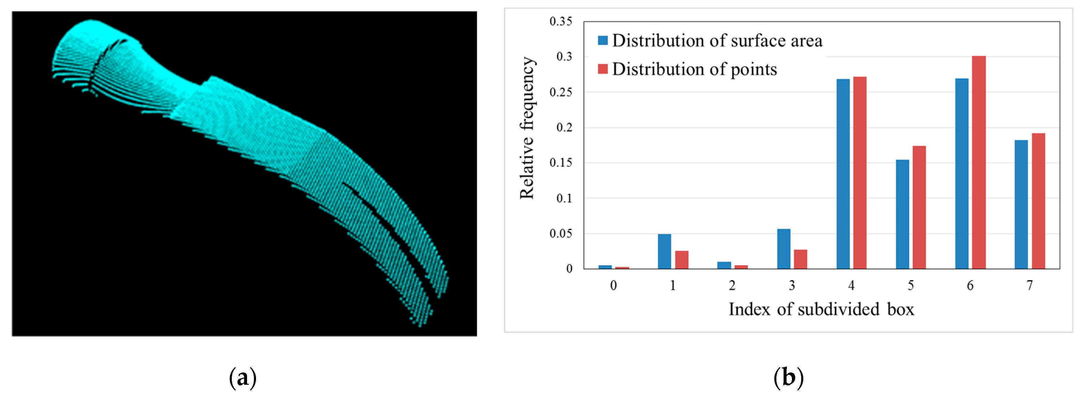
Equation (5) is the simplified regional area-based descriptor. The descriptor captures less precise information included in the surface area-based descriptor, but it still retains most of the discriminative power of the surface area-based descriptor. The regional area-based descriptor and its simplification are shown in Figure 8b. As can be seen, the distribution of the surface area inside the OBB of the object in this case is almost the same as the distribution of points inside the OBB. Furthermore, the efficiency of simplification is demonstrated by six tests in Figure 9.

2.3. D Virtual Camera

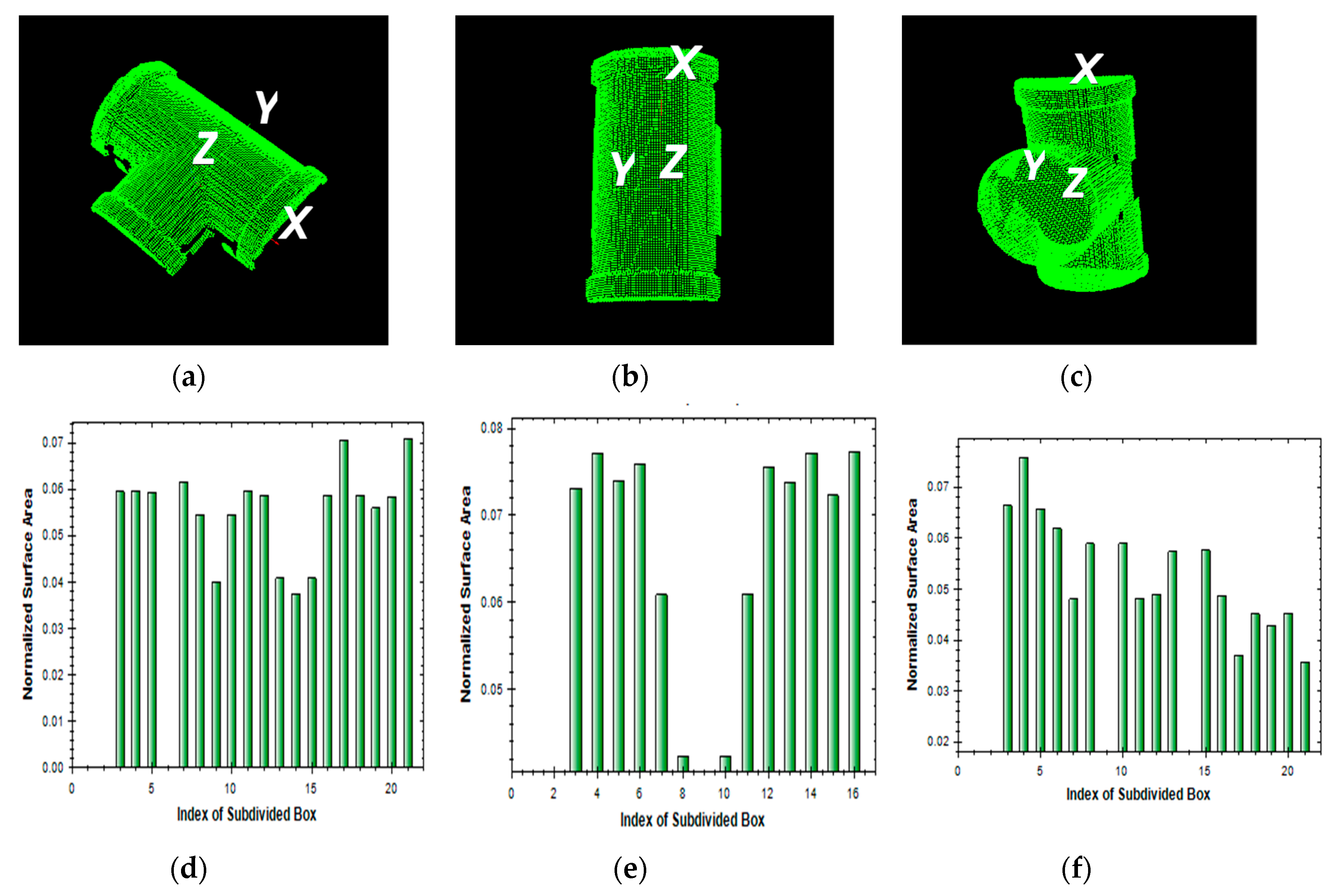
A virtual sensor is developed to extract the template point clouds corresponding to various views of the model. The virtual sensor with the same internal properties as the real one is located at the origin of the world coordinate system. The central axis of the virtual camera is defined as the z-axis. The CAD model of the object is positioned on the z-axis. The working distance, tz, is shown in Figure 10. The reference point clouds are generated by rotating the model around the x-axis with every increment θx and around the y-axis with every increment θy. For each rotation, a set of point clouds is created corresponding to one view of the model. Figure 11 shows the different views of the CAD model in Figure 10.

2.4. Feature Matching

Given a feature vector FVO that represents the object point clouds O, the matched feature vector FVM that represents a view of the model needs to be estimated. The feature vector FVM is built through the database generation process in the offline phase. The feature vector FV comprises the OBB parameters and the regional area-based descriptor. In the first step, the OBB parameters between the object point clouds and the object model are compared for best matching from a series of viewpoints [30]. When the OBB matching result satisfies the preset condition, the regional area-based descriptor between the object point clouds is then matched with the object model defined from the viewpoint. The general process for matching the object point clouds with the model is shown in Figure 12.

2.4.1. OBB Matching

The OBB matching process determines the views of the object model comprising the same dimensions as the object point clouds. The OBB of each template point cloud is represented by three vectors, including CCM1(xMmax, yMmax, zMmax), CCM2(xMmid, yMmid, zMmid), and CCM3(xMmin, yMmin, zMmin), while the OBB of the object point clouds is denoted by CC1(xmax, ymax, zmax), CC2(xmid, ymid, zmid), and CC3(xmin, ymin, zmin), respectively. These two OBBs should be satisfied by the following equation:
d c o r r = 1 3 ( C C M 1 C C 1 C C M 1 + C C M 2 C C 2 C C M 2 + C C M 3 C C 3 C C M 3 ) < d t h r e s h ,
where dthresh is the given adequate threshold.

2.4.2. Matching Criteria for Regional Area-based Descriptor

The regional area-based descriptor presents the histogram of the surface area of the object. The resemblance between the object and model descriptors is measured using NCC. Let FO = {fv, v = 0, …, nV} be the regional area-based descriptor of the object point clouds and FM = {fMv, v = 0, …, nV} be the regional area-based descriptor of the template point clouds. The NCC between FO and FM is computed as follows:
C ( F O , F M ) = v = 0 n V ( f v f ¯ ) ( f M v f ¯ M ) v = 0 n V ( f v f ¯ ) 2 v = 0 n V ( f M v f ¯ M ) 2 ,
where f ¯ = 1 n V + 1 v = 0 n V f v and f ¯ M = 1 n V + 1 v = 0 n V f M v .
If the coefficient C(FO, FM) is larger than a given threshold, the matching result is good and the two feature vectors FVO and FVM can be adopted to estimate the initial transformation matrix between the object point clouds and the model.

2.4.3. Transformation Estimation and Refinement

Through the matching step, the correspondence feature vectors FVO and FVM are obtained. According to these feature vectors, the initial transformation matrix Tinitial between the object point clouds and the model can be estimated by aligning the frame {CM, vM1, vM2, vM3} that represents the model to the frame {C, v1, v2, v3} that represents the object point clouds.
[ x C x C + v 11 x C + v 21 x C + v 31 y C y C + v 12 y C + v 22 y C + v 32 z C z C + v 13 z C + v 23 z C + v 33 1 1 1 1 ] = T i n i t i a l [ x M C x M C + v M 11 x M C + v M 21 x M C + v M 31 y M C y M C + v M 12 y M C + v M 22 y M C + v M 32 z M C z M C + v M 13 z M C + v M 23 z M C + v M 33 1 1 1 1 ]
The accuracy of initial pose estimation is limited by the set of templates in the database. Each template describes only one view of the object and the number of templates is restricted; hence, the matched template may not be exactly the same as the detected object. For example, some small parts of the detected object are missed from the template. Hence, the estimated 3-D pose may be incorrect. Additionally, the measurement data can lose some high-frequency information (such as the edges of the object) owing to limitation of the measurement system. The measurement errors can reduce the accuracy of the initial 3-D pose estimation. Therefore, it is necessary to refine the estimated initial 3-D pose. The algorithm often performed to obtain the refined transformation is the ICP algorithm [32,33]. The ICP algorithm is a matching process that minimizes the fitting deviation between two matching point clouds, and iteratively refines the transformation through minimizing the distance between the points of the object point clouds and the model. The steps of the ICP algorithm are described as follows:
  • For each point pO, find the closest point qM;
  • Estimate the rotation matrix R and translation vector t that minimize the root mean squared distance;
  • Transform Ok+1Q(Ok) using the estimated parameters;
  • Terminate the iteration when the change in error falls below the preset threshold.

3. Experimental Results and Analysis

The feasibility of the proposed methodology is verified by comparing simulated and actual data obtained from experiments on industrial objects. Figure 13 shows the experimental setup for the robot pick and place application that involves the regional area-based descriptor. The developed 3-D scanner has been integrated with the robotic arm to acquire the 3-D point clouds that represent the randomly stacked objects in the scene. The measurement volume of the 3-D scanner is approximately 147 × 110 × 80 mm3. The simulation data provided by Industrial Technology Research Institute (ITRI) comprise the database of six different work parts. The dimensions of each object in the ITRI database are shown in Table 1. The resolution of the scene point clouds in the database is greater than 0.5 mm. Actual data are measured using the developed 3-D optical scanner according to the random speckle pattern projection principle and the triangulation theory. The depth resolution of the measured data is about 0.3 mm and the spatial resolution is 1.05 mm. In the experiment, the datasets are processed on a computer with a Core i5 processor (3.40 GHz and 4 GB RAM).
A viewpoint is defined as a set of six parameters, with three position parameters (x, y, z) defining the spatial position of the 3-D sensor, and three orientation parameters (Rx, Ry, Rz) defining the direction of the sensor. The accuracy of a point cloud in the measurement using the 3-D sensor depends on the angle of incidence of the sensor on the surface. The ideal angle is π/2; that is, the closer the angle of incidence of the sensor is to the normal surface direction, the more accurate the measured points. To ensure quality of the measured data, a quality criterion is included in the experimental system. This criterion states that acquired point clouds detected using local normal vectors should satisfy a uniform distribution condition. Therefore, the simplified regional area-based descriptor is utilized for all tested data.

3.1. Case Study on Simulated Data

In testing the simulation data, Gaussian random noise is added to the object point clouds with increasing standard deviation on σ from 0.001 to 1.0. Following this, the object descriptor is compared with the descriptors of the templates to determine the correlation coefficient using Equation (7). For each model, the correlation coefficient corresponding to each Gaussian noise level is the average of 30 values, which measure the similarity between 30 different object point clouds with the model. The accuracy of the proposed method is evaluated by determining the root mean squares (RMS), translation, and rotation errors. In addition, the computation time of the object recognition and localization process is measured to evaluate the efficiency of the proposed method.
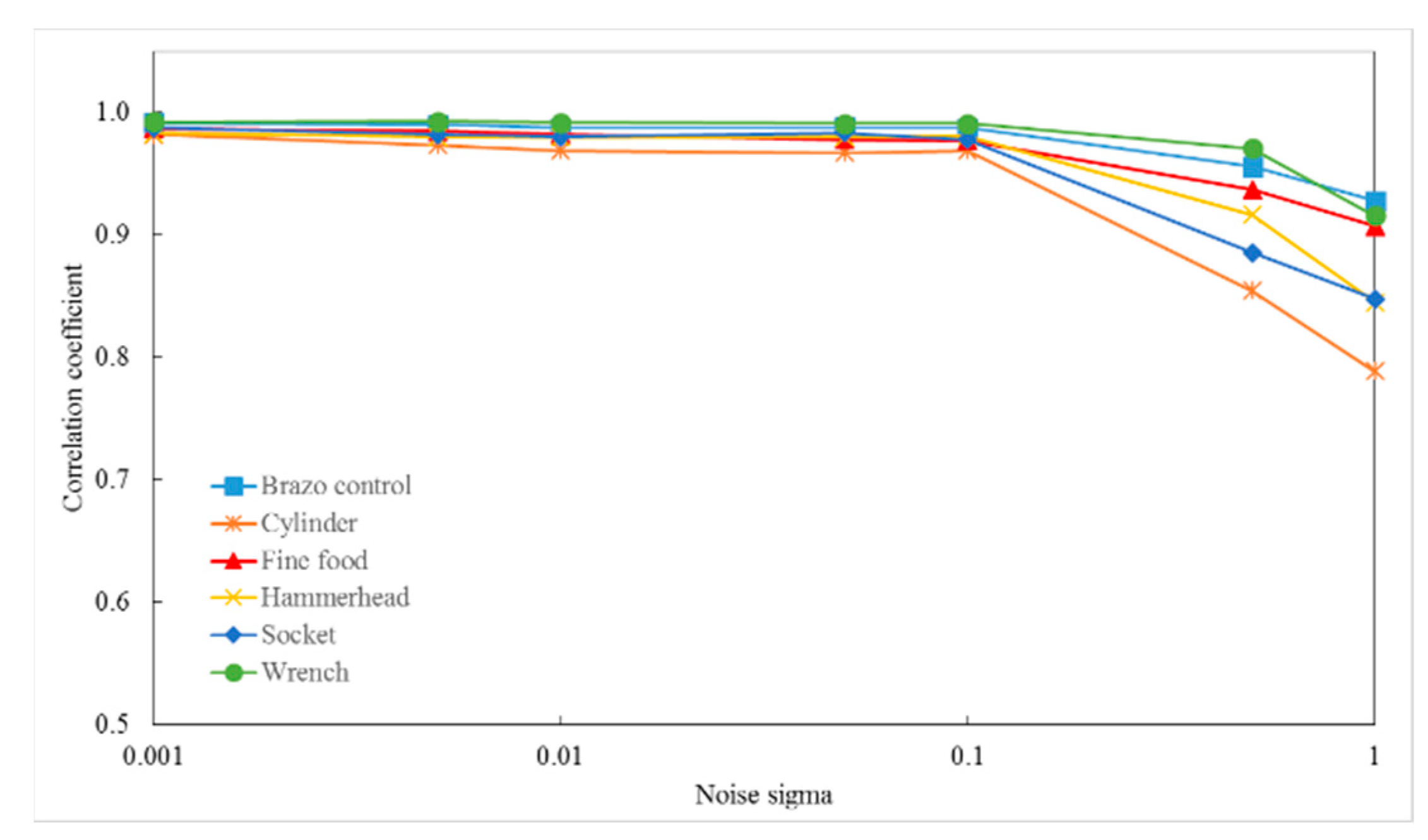
Figure 14 shows examples of input object point clouds with different Gaussian noise levels. The effect of Gaussian noise on matching between the object descriptor and model descriptor is illustrated in Figure 15. In this experiment, the correlation coefficients obtained can exceed 0.8 with a noise level of σ below 1.0.
The accuracy of the 3-D object recognition and localization algorithm can be evaluated by RMS, translation, and rotation errors. The RMS error is calculated using the distance between corresponding points in the CAD model (pitrue) and transformed point clouds (pialg) under the estimated transformation matrix. Translation error (Terr) is the absolute difference between the true and computed translation vectors (Ttrue and Talg). Rotation error (qerr) is the absolute difference between the true and computed unit quaternions (qtrue and qalg) representing the rotations of objects in 3-D space.
T e r r = T a l g T t r u e ,
q e r r = q a l g q t r u e ,
R M S e r r = i = 1 n ( p i a l g p i t r u e ) 2 n .
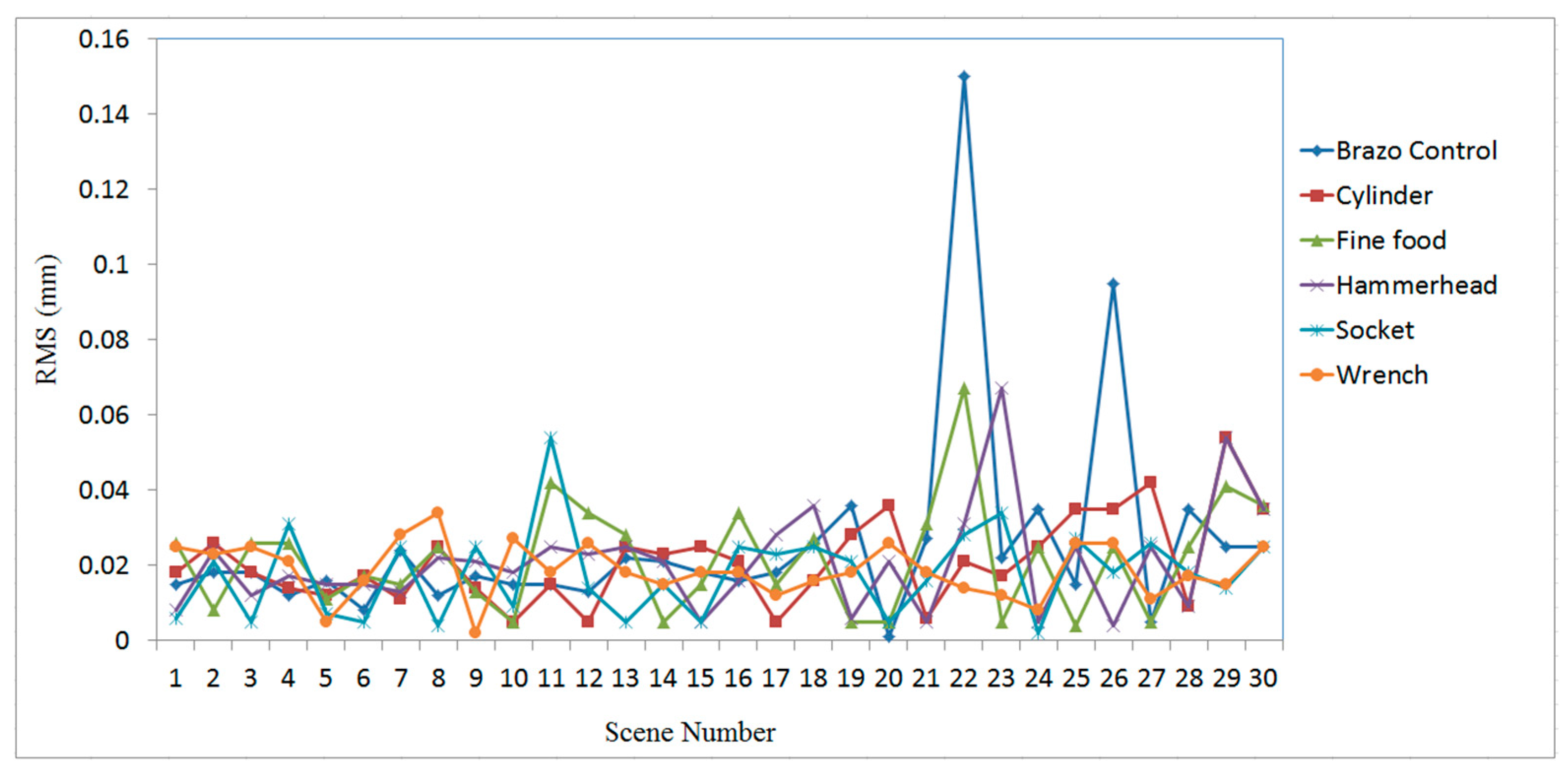
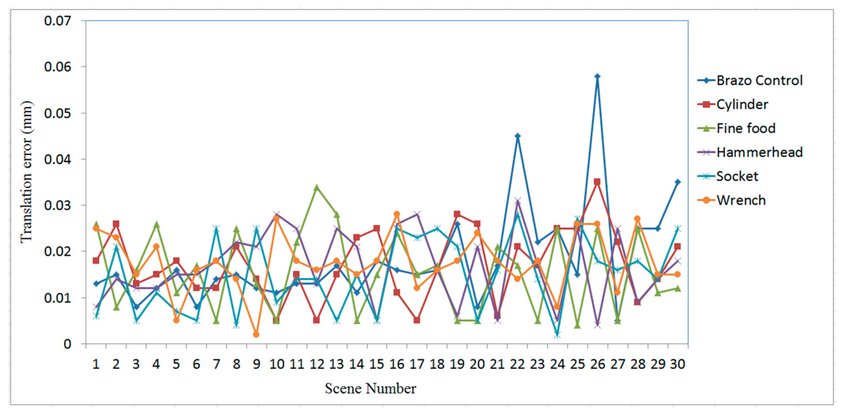
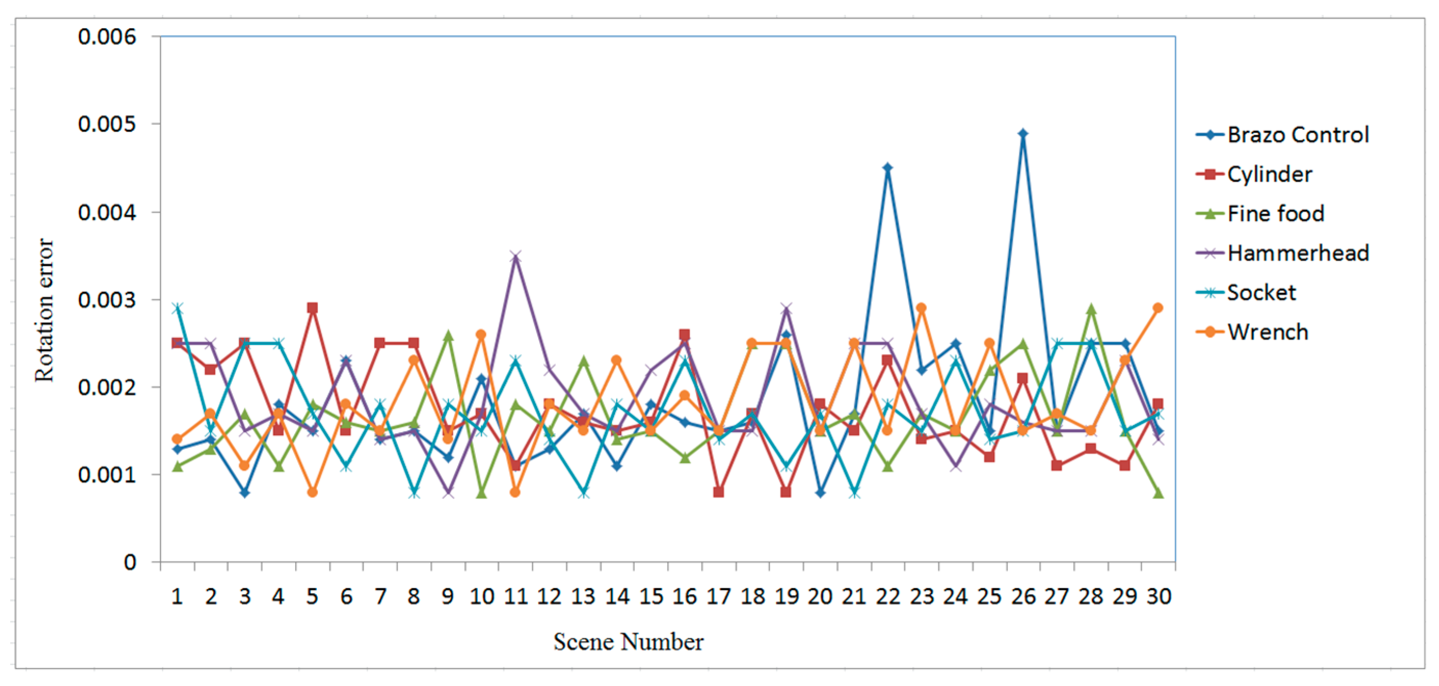
Figure 16, Figure 17 and Figure 18 show the RMS, translation, and rotation errors, respectively, of six different types of objects in the ITRI (Industrial Technology Research Institute) database. The maximum RMS error is smaller than 0.15 mm. The translation errors do not exceed 0.06 mm. In addition, the rotation errors are smaller than 0.005°.
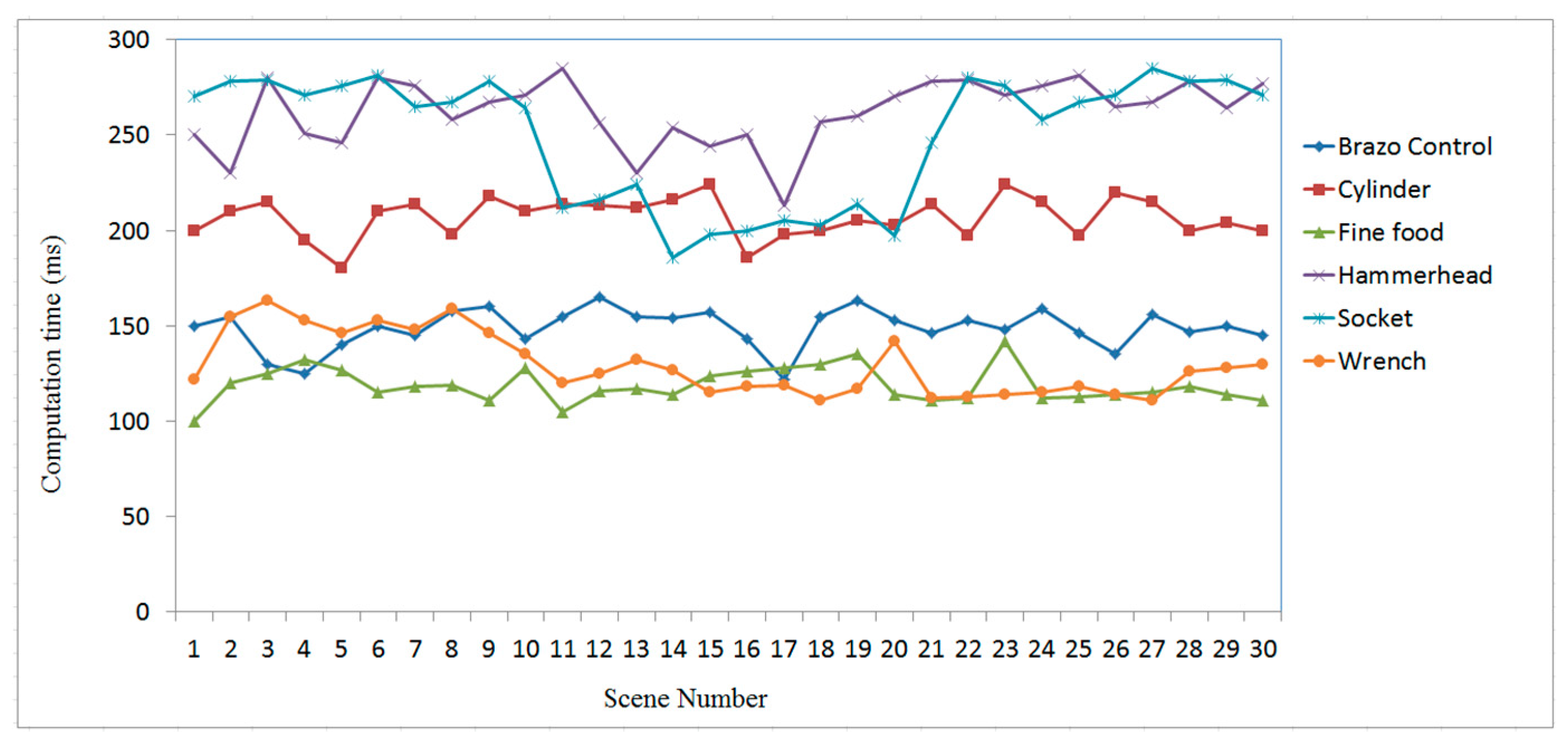
To evaluate the efficiency of the proposed recognition and localization algorithm, the simplified regional area-based descriptor is employed. This descriptor captures less precise information included in the surface area-based descriptor, but it retains most of the discriminative power of the regional area-based descriptor. The computation time of the object recognition and localization tasks is summarized in Figure 19. The average time required to recognize and localize the object is less than 0.3 s for all tested objects.
The comparison of performances between the proposed approach and existing methods is reported in Table 2. As can be seen, the developed method outperforms in pose estimation accuracy and computation cost. In terms of computational efficiency, it is worth noting that the benefits of speed offered by the proposed method outweigh the others. Thus, regional area-based object recognition and the localization algorithm can achieve a real-time and accurate pose estimation of 3D objects in cluttered range images.

3.2. Case Study on Measured Data

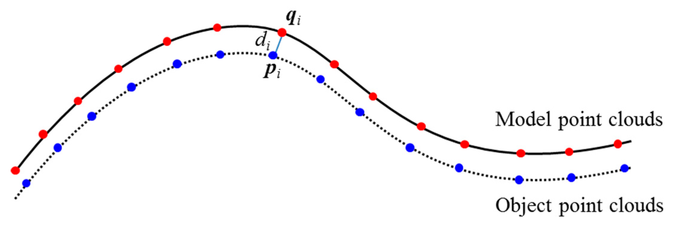
In the experiments with the measured data, different types of objects were selected to test the effectiveness of the proposed algorithm. The samples are randomly stacked on the table to ensure randomness in their positions and orientations. The performance of object matching can be evaluated by judging the distance from each point in the measured cloud to the closest point in the model [34]. Denote di as the distance between a point (pi) in the measured cloud and its closest point (qi) in the model (shown in Figure 20). Then, the mean distance, μ, and standard deviation, σ, can be computed to evaluate the matching condition as follows:
μ = 1 n i = 1 n d i ,
σ = i = 1 n ( d i μ ) 2 n 1 ,
where n is the number of points in the measured point clouds.
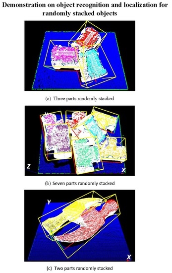
As seen in Figure 21, the location and orientation of all objects can be effectively detected by using the developed method. Three experimental cases are shown, in which three, seven, and two various parts are contained in each case, respectively, for object recognition and localization. The correlation coefficients in the matching process are higher than 0.9. For all tested data, the localization of each part can be completed within 0.5 s. In addition, the mean deviation ranges between 0.180 mm and 0.469 mm and the standard deviation ranges between 0.168 mm and 0.484 mm (shown in Table 3).
In Figure 22, two cases were further tested for the verification of handling more complexity. Case 1 has five parts with an objective to detect a connector, while Case 2 has five parts with an objective to detect a 3D-printed hammer. By using the developed method, two connectors were effectively detected with part orientation determined in Case 1. In Case 2, the 3D-printing hammer, which is partly overlapped by a toy model, can also be detected effectively with its orientation localized.

4. Discussion

The proposed methods have been implemented and tested on non-overlapping, multiple overlapping, and stacked objects in 3-D scene point clouds. In this section, the advantages and limitations of object recognition and localization are discussed. The developed method represents the object in 3-D space based on the distribution of the object’s surface area inside the OBB. Surface area is an intrinsic surface property and independent of surface sampling; hence, the developed feature descriptor is invariant to arbitrary rotations and translations of the object. In addition, the feature descriptor is less sensitive to surface sampling and noise. As illustrated in Figure 15, the correlation coefficients exceed 0.8 with a noise level σ equal to 1.0.
The effectiveness and accuracy of the proposed 3-D object recognition and localization have been tested on both simulated and measured data. The accuracy of the proposed method in the experiment with simulated data is evaluated in terms of RMS, translation, and rotation errors, which were found to be below 0.15 mm, 0.06 mm, and 0.005°, respectively.
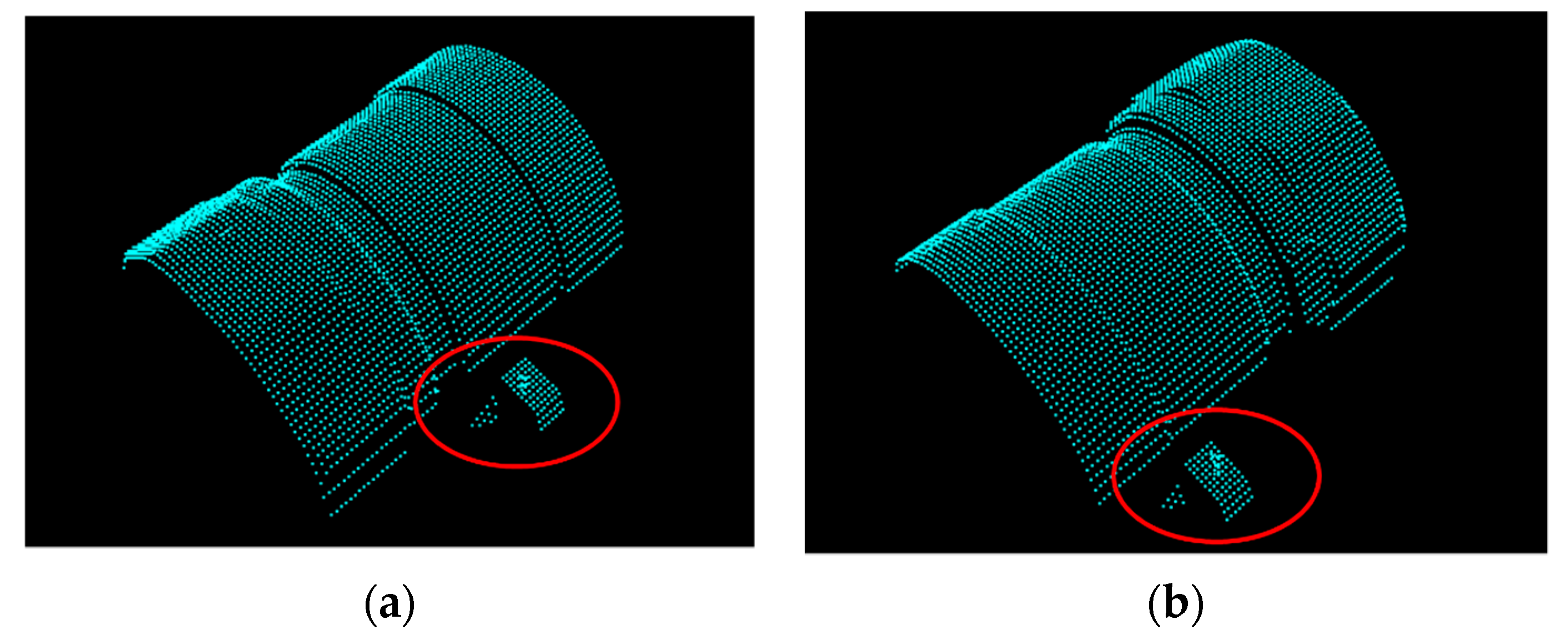
The proposed algorithm employs a point-to-point ICP algorithm to match the scene point clouds with the model; hence, the accuracy can be affected by the resolution of the scene point clouds, which is about 0.5 mm in the experiment. Therefore, some important features of the object located in the small surface regions are only represented by a small number of measured points, thus causing errors when estimating the position and orientation of the target object. For example, the scene nos. 19 and 28 of the finefood object shown in Figure 23, respectively, are only represented by a rather small number of point clouds. Due to this reason, the RMS and rotation errors of scene nos. 19 and 28 of the finefood object shown in Figure 16 (in Page 15) and Figure 18 (in Page 16), respectively, are larger than those of the other scenes.
Errors in the initial transformation estimation process depend considerably on the rotation increments θx and θy of templates generated by the virtual camera. To enhance the matching accuracy, the rotation increment is controlled to be smaller. However, a smaller increment can easily generate a significant increase in the runtime of the operation process. Take for instance an experiment having 10,000 points, such as Wrench shown in Table 2; its computation time in the case θx = θx = 0.157 (rad) was 3 s, which is much longer than that in the case θx = θx = 0.785 0.157 (rad), at merely 0.15 s.
In the experiment with the actual measurement data, the accuracy of the proposed method is estimated according to the matching deviation between the object point clouds and the model. The performance of object matching is evaluated using the mean distance and its standard deviation. With the measured point clouds having a depth resolution of 0.3 mm and spatial resolution of 1.05 × 1.05 mm2, the proposed method can achieve a mean deviation below 0.47 mm and standard deviation below 0.49 mm. To increase the accuracy of the developed algorithm, the best way is to improve the quality and resolution of the measured point clouds.
The efficiency of the 3-D object recognition and localization algorithm is a very important parameter for the 3-D vision system in practical applications. In the experiment, for a set of more than 16k points in one 3-D image map, the proposed method requires only 0.5 s for each recognized object using a common PC, and it can be reduced to 0.1 s by simplification. To substitute it for a regional area-based descriptor, the measured point cloud is required to have a certain level of density and uniform distribution. The computation cost of the algorithm is proved to be efficient for in-line industrial automation.

5. Conclusions

In this study, a new method for automated 3-D object recognition and localization has been developed using 3-D point clouds. Experimental results indicate the effectiveness of the proposed method. In addition, the developed approach can accurately detect the position and orientation of the target objects, which are randomly stacked in an unstructured bin. The detection accuracy is affected by the spatial and depth resolution of the measured point cloud. The proposed method can achieve a localization accuracy better than half of the spatial resolution of the point cloud. The developed algorithm would be particularly useful for the automation of workpiece manipulation and handling in manufacturing sectors. Enhancement of computational efficiency of the object recognition process is achievable by further employing parallel computing techniques.

Author Contributions

Conceptualization, L.C.-C.; Methodology, L.C.-C. and T.-H.N.; Software, T.-H.N.; Validation, L.C.-C. and T.-H.N.; Formal Analysis, L.C.-C. and T.-H.N.; Investigation, L.C.-C. and T.-H.N.; Resources, L.C.-C.; Data Curation, L.C.-C. and T.-H.N.; Writing—Original Draft Preparation, L.C.-C. and T.-H.N.; Writing—Review & Editing, L.C.-C.; Visualization, L.C.-C.; Supervision, L.C.-C.; Project Administration, L.C.-C.; Funding Acquisition, L.C.-C.

Funding

This research was funded by Ministry of Science and Technology, Taiwan, under grant no. MOST 107-2218-E-002-060.

Conflicts of Interest

The authors declare no conflict of interest.

References

  1. Birk, J.R.; Kelley, R.B.; Martins, H.A.S. An orienting robot for feeding workpieces stored in bins. IEEE Trans. Syst. Man Cybern. 1981, 11, 151–160. [Google Scholar] [CrossRef]
  2. Kelley, R.B.; Birk, J.R.; Martins, H.A.S.; Tella, R. A robot system which acquires cylindrical workpieces from bins. IEEE Trans. Syst. Man Cybern. 1982, 12, 204–213. [Google Scholar] [CrossRef]
  3. Torgerson, E.; Paul, F.W. Vision-guided robotic fabric manipulation for apparel manufacturing. IEEE Control Syst. Mag. 1988, 8, 14–20. [Google Scholar] [CrossRef]
  4. Cai, C.; Regtien, P.P.L. A smart sonar object recognition system for robots. Meas. Sci. Technol. 1993, 4, 95–100. [Google Scholar] [CrossRef]
  5. Kuehnle, J.; Verl, A.; Xue, Z.; Ruehl, S.; Zoellner, J.M.; Dillmann, R.; Grundmann, T.; Eidenberg, R.; Zoellner, R.D. 6D Object Localization and Obstacle Detection for Collision-Free Manipulation with a Mobile Service Robot. In Proceedings of the International Conference on Advanced Robotics, Munich, Germany, 22–26 June 2009; pp. 1–6. [Google Scholar]
  6. Fuchs, S.; Haddadin, S.; Keller, M.; Parusel, S.; Kolb, A.; Suppa, M. Cooperative Bin-Picking with Time-of-Flight Camera and Impedance Controlled DLR Lightweight Robot III. In Proceedings of the IEEE/RSJ International Conference on Intelligent Robots and Systems, Taipei, Taiwan, 18–22 October 2010; pp. 4862–4867. [Google Scholar]
  7. Skotheim, O.; Thielemann, J.T.; Berge, A.; Sommerfelt, A. Robust 3D Object Localization and Pose Estimation for Random Bin Picking with the 3DMaMa Algorithm. In Proceedings of the SPIE 7526 Three-Dimensional Image Processing and Application, San Jose, CA, USA, 4 February 2010; Volume 7526, p. 75260E. [Google Scholar]
  8. Liu, M.-Y.; Tuzel, O.; Veeraraghavan, A.; Taguchi, Y.; Marks, T.K.; Chellappa, R. Fast object localization and pose estimation in heavy clutter for robotic bin picking. Int. J. Rob. Res. 2012, 32, 951–973. [Google Scholar] [CrossRef]
  9. Skotheim, O.; Lind, M.; Ystgaard, P.; Fjerdingen, S.A. A Flexible 3D Object Localization System for Industrial Part Handling. Int. Robot. Syst. (IROS). In Proceedings of the IEEE/RSJ International Conference, Vilamoura, Portugal, 7–12 October 2012; pp. 3326–3333. [Google Scholar]
  10. Nieuwenhuisen, M.; Droeschel, D.; Holz, D.; Stuckler, J.; Berner, A.; Li, J.; Klein, R. Mobile Bin Picking with an Anthropomorphic Service Robot. In Proceedings of the IEEE International Conference on Robotics and Automation, Karlsruhe, Germany, 6–10 May 2013; pp. 2327–2334. [Google Scholar]
  11. Sansoni, G.; Bellandi, P.; Leoni, F.; Docchio, F. Optoranger: A 3D pattern matching method for bin picking applications. Opt. Lasers Eng. 2014, 54, 22–231. [Google Scholar] [CrossRef]
  12. Schnabel, R.; Wessel, R.; Wahl, R.; Klein, R. Shape Recognition in 3D Point-Clouds. In Proceedings of the 16th International Conference in Central Europe on Computer Graphics Visualization and Computer Vision, Plzen, Czech Republic, 4–7 February 2008. [Google Scholar]
  13. Johnson, A.E.; Hebert, M. Surface matching for object recognition in complex three-dimensional scenes. Image Vis Comput. 1998, 16, 635–651. [Google Scholar] [CrossRef]
  14. Chen, H.; Bhanu, B. 3D free-form object recognition in range images using local surface patches. Pattern Recogn. Lett. 2007, 28, 1252–1262. [Google Scholar] [CrossRef]
  15. Zaharescu, A.; Boyer, E.; Varanasi, K.; Horaud, R. Surface Feature Detection and Description with Applications to Mesh Matching. In Proceedings of the IEEE Conference on Computer Vision adn Pattern Recognition, Miami, FL, USA, 20–25 June 2009; pp. 373–380. [Google Scholar]
  16. Drost, B.; Ulrich, M.; Navab, N.; Ilic, S. Model Globally, Match Locally: Efficient and Robust 3D Object Recognition. In Proceedings of the IEEE Conference on Computer Vision and Pattern Recognition, San Francisco, CA, USA, 13–18 June 2010; pp. 998–1005. [Google Scholar]
  17. Rusu, R.B.; Bradski, G.; Thibaux, R.; Hsu, J. Fast 3D recognition and pose using the Viewpoint Feature Histogram. In Proceedings of the IEEE/RSJ International Conference on Intelligent Robots and System, Taipei, Taiwan, 18–22 October 2010; pp. 2155–2162. [Google Scholar]
  18. Salti, S.; Tombari, F.; Di Stefano, L. SHOT: Unique signatures of histograms for surface and texture description. Comput. Vis Image Underst. 2014, 125, 251–264. [Google Scholar] [CrossRef]
  19. Le, V.-H.; Le, T.-L.; Vu, H.; Nguyen, T.T.; Tran, T.-H.; Dao, T.-C.; Nguyen, H.-Q. Geometry-Based 3D Object Fitting and Localizing in Grasping Aid for Visually Impaired. In Proceedings of the IEEE Interntional Conference on Consumer Electronics (ICCE), Mumbai, India, 7–11 January 2016; p. 1. [Google Scholar]
  20. Dantanarayana, H.G.; Huntley, J.M. Object recognition and localization from 3D point clouds by maximum-likelihood estimation. R Soc. Open Sci. 2017, 4, 160693. [Google Scholar] [CrossRef] [PubMed]
  21. Chen, L.-C.; Hong, H.; Nguyen, X.-L.; Wu, H.-W. Novel 3-D object recognition methodology employing a curvature-based histogram. Int. J. Adv. Robot Syst. 2013. [Google Scholar] [CrossRef]
  22. Chen, L.-C.; Nguyen, T.-H.; Lin, S.-T. Viewpoint-independent. 3D object segmentation for randomly stacked objects using optical object detection. Meas. Sci. Technol. 2015, 26, 105202. [Google Scholar]
  23. Rabbani, T.; van den Heuvel, F.A.; Vosselman, G. Segmentation of point clouds using smoothness constraint. Int. Arch. Photogramm. Remote Sens. Spat. Inf. Sci. 2006, 35, 248–253. [Google Scholar]
  24. Nurunnabi, A.; Belton, D.; West, G. Robust Segmentation in Laser Scanning 3D Point Cloud Data. In Proceedings of the International Conference on Digital Image Computing Techniques and Applications, Fremantle, WA, Australia, 2–5 December 2012; pp. 1–8. [Google Scholar]
  25. Rusu, R.B.; Blodow, N.; Marton, Z.C.; Beetz, M. Close-Range Scene Segmentation and Reconstruction of 3D Point Cloud Maps for Mobile Manipulation in Domestic Environments. In Proceedings of the IEEE/RSJ International Conference on Intelligent Robots and Systems, St. Louis, MO, USA, 10–15 October 2009; pp. 1–6. [Google Scholar]
  26. Douillard, B.; Underwood, J.; Kuntz, N.; Vlaskine, V.; Quadros, A.; Morton, P.; Frenkel, A. On the Segmentation of 3D LIDAR Point Clouds. In Proceedings of the IEEE International Conference on. Robotics and Automation, Shanghai, China, 9–13 May 2011; pp. 2798–2805. [Google Scholar]
  27. Anguelov, D.; Taskarf, B.; Chatalbashev, V.; Koller, D.; Gupta, D.; Heitz, G.; Ng, A. Discriminative Learning of Markov Random Fields for Segmentation of 3D Scan Data. In Proceedings of the IEEE Computer Society Conference on Computer Vision and Pattern Recognition, San Diego, CA, USA, 20–25 June 2005; Volume 2, pp. 169–176. [Google Scholar]
  28. Golovinskiy, A.; Funkhouser, T. Min-Cut Based Segmentation of Point Clouds. In Proceedings of the IEEE International Conference on Computer Vision and Workshop, Kyoto Japan, 27 September–4 October 2009; pp. 39–46. [Google Scholar]
  29. Munoz, D.; Vandapel, N.; Hebert, M. Onboard Contextual Classification of 3-D Point Clouds with Learned High-Order Markov Random Fields. In Proceedings of the IEEE International Conference on Robotics an Automation, Kobe, Japan, 12–17 May 2009; pp. 2009–2016. [Google Scholar]
  30. Chen, L.-C.; Hoang, D.-C.; Lin, H.-I.; Nguyen, T.-H. Innovative methodology for multi-view point clouds registration in robotic 3-D object scanning and reconstruction. Appl. Sci. 2016, 6, 132. [Google Scholar] [CrossRef]
  31. Gottschalk, S.; Lin, M.C.; Manocha, D. OBBTree: A Hierarchical Structure for Rapid Interference Detection. In Proceedings of the 23rd Annual Conference on Computer Graphics and Interactive Technique, New Orleans, LA, USA, 4–9 August 1996; pp. 171–180. [Google Scholar]
  32. Besl, P.J.; McKay, N.D. A method for registration of 3-D shapes. IEEE Trans. Pattern. Anal. Mach. Intell. 1992, 14, 239–256. [Google Scholar] [CrossRef]
  33. Marton, Z.C.; Rusu, R.B.; Beetz, M. On Fast Surface Reconstruction Methods for Large and Noisy Point clouds. In Proceedings of the IEEE International Conference on Robotics and Automation, Kobe, Japan, 12–17 May 2009; pp. 3218–3223. [Google Scholar]
  34. Krebs, B.; Sieverding, P.; Korn, B. A Fuzzy ICP Algorithm for 3D Free-Form Object Recognition. In Proceedings of the 13th International Conference on Pattern Recognition, Vienna, Austria, 25–29 August 1996; Volume 1, pp. 539–543. [Google Scholar]
Figure 1. Overview of 3-D object recognition and localization.
Sensors 19 00764 g001
Figure 2. Flowchart of the proposed 3D object recognition and localization algorithm.
Sensors 19 00764 g002
Figure 3. Principle of the proposed 3-D object segmentation method. (a) Measured point clouds. (b) Distance map. (c) Generated markers. (d) Segmentation result of 3-D point clouds.
Sensors 19 00764 g003
Figure 4. Oriented bounding box of segmented point clouds.
Sensors 19 00764 g004
Figure 5. OBB of object subdivided into n (= k1 × k2 × k3) sub-boxes.
Sensors 19 00764 g005
Figure 6. Regional area-based descriptor. (a) Object point clouds. (b) Regional area-based descriptor of the object.
Sensors 19 00764 g006
Figure 7. An example of regional area-based descriptor of an L-shape object with different number of subdivided boxes in OBB n = k1 × k2 × k3 (a) point cloud; (b) k1 × k2 × k3 = 5 × 5 × 1; (c) k1 × k2 × k3 = 5 × 4 × 3; (d) k1 × k2 × k3 = 5 × 5 × 4.
Sensors 19 00764 g007
Figure 8. Distribution of surface area and points inside the OBB of the object. (a) Object point clouds. (b) Regional area-based descriptor of the object (blue) and its simplification (red).
Sensors 19 00764 g008
Figure 9. Comparison of computation time between original regional area-based descriptor and simplified descriptor inside OBBs of six point clouds.
Sensors 19 00764 g009
Figure 10. Virtual camera and model.
Sensors 19 00764 g010
Figure 11. 3D virtual sensor. (ac) Point clouds corresponding to various views of the model; (df) regional area-based descriptors of point clouds of (ac) cases, respectively.
Sensors 19 00764 g011
Figure 12. Flowchart for matching object point clouds with the model.
Sensors 19 00764 g012
Figure 13. System setup for pick and place application using regional area-based descriptor.
Sensors 19 00764 g013
Figure 14. Object point clouds with Gaussian noise added and standard deviation of 0.001, 0.05, and 1.0.
Sensors 19 00764 g014
Figure 15. Effect of Gaussian noise on matching between object descriptor and model descriptor.
Sensors 19 00764 g015
Figure 16. RMS errors obtained using the proposed algorithm for different types of objects in ITRI database.
Sensors 19 00764 g016
Figure 17. Translation errors obtained using the proposed algorithm for different types of objects in ITRI database.
Sensors 19 00764 g017
Figure 18. Rotation errors obtained using the proposed algorithm for different types of objects in ITRI database.
Sensors 19 00764 g018
Figure 19. Time consumed for 3-D object recognition and localization using the proposed algorithm.
Sensors 19 00764 g019
Figure 20. Query point pi in measured point clouds and its nearest point, qi, in the model.
Sensors 19 00764 g020
Figure 21. Object recognition and localization results for different types of objects: (a) three parts randomly stacked; (b) seven parts randomly stacked and (c) two parts randomly stacked.
Sensors 19 00764 g021
Figure 22. Example of measurement using the NTU-3D Probe: (a,d) show acquired speckle images; (b,e) show acquired 3D point clouds; (c,f) show object recognition and localization results.
Sensors 19 00764 g022
Figure 23. Two views of finefood model in ITRI database. (a) Scene no. 19 and (b) Scene no. 28.
Sensors 19 00764 g023
Table 1. Dimensions of objects in ITRI database.
ModelDimensions (mm)
Name3-D representationLengthWidthHeight
Brazo control Sensors 19 00764 i001865330
Cylinder Sensors 19 00764 i002353535
Finefood Sensors 19 00764 i003414033
Hammerhead Sensors 19 00764 i00411035.522
Socket Sensors 19 00764 i005453535
Wrench Sensors 19 00764 i0061546513.2
Table 2. A comparison of performances obtained by the proposed method and existing methods on simulated data.
ModelsMethodTranslation Error (mm)Rotation Error (10−3 rad)Time (s)
Fine foodGraph-based0.8690.1032.537
Feature-based 0.4120.0721.453
View-based0.0360.0877.521
Proposed0.0190.0680.160
CylinderGraph-based0.4350.1454.896
Feature-based 0.1320.7682.902
View-based0.0380.1088.247
Proposed0.0220.0610.182
WrenchGraph-based0.2130.3154.184
Feature-based 0.8960.9793.262
View-based0.0780.1139.163
Proposed0.0170.0810.150
Table 3. Matching performance for objects in Figure 21.
Case studyObjectMatching Score (%)Mean Deviation µ (mm)Standard Deviation σ (mm)
1Red89.740.3200.392
Magenta 90.120.3890.426
Cyan85.550.4690.484
2Red98.770.2490.313
Yellow99.230.1870.242
Magenta97.550.2470.316
Cyan92.880.3510.431
Purple91.740.3290.394
Gold98.550.2310.305
Spring green94.570.3130.372
3Red98.310.2660.264
Yellow99.260.1800.168
Average:94.690.2940.342