5.1. Validation of Deflection Calculation
The comparison between the static and dynamic test results under different cases was performed to validate the correctness and efficiency of the bridge deflection calculation method based on the modal theory and the improved Kriging method. The deflection results of three measure points are described in
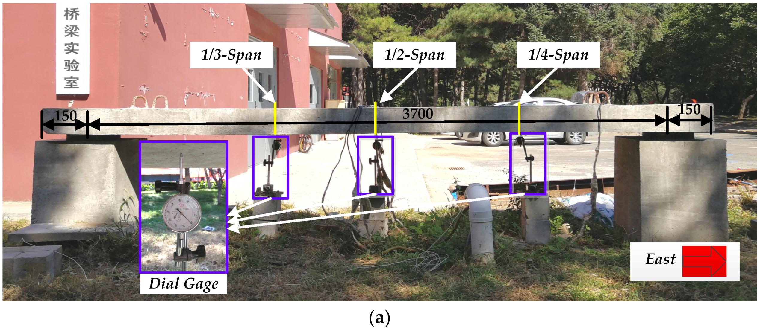
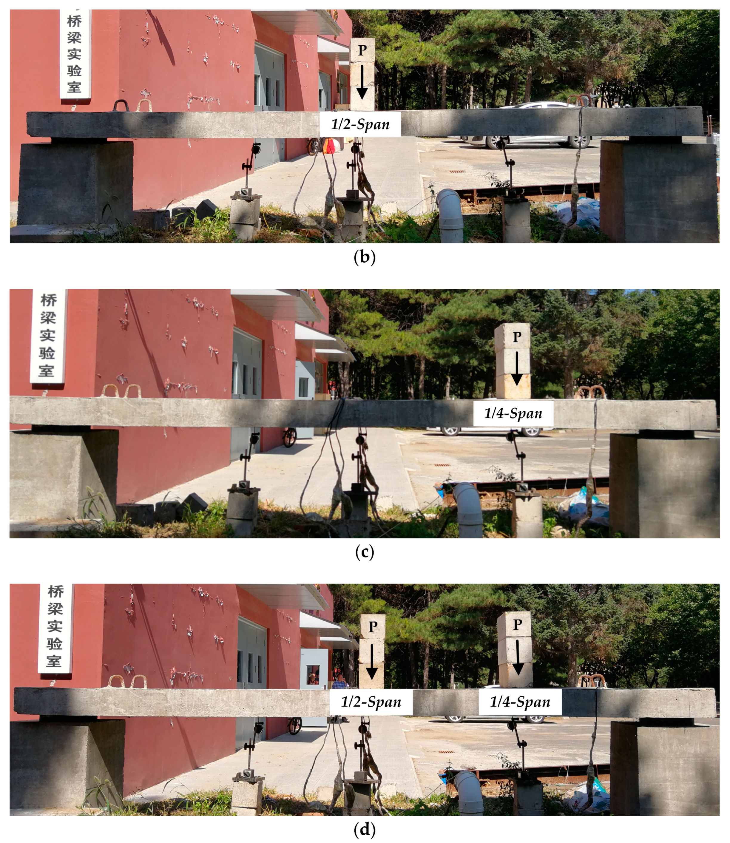
Table 2. For each case, the deflections at 1/4-Span, 1/2-Span, and 1/3-Span were all measured four times. Although the deflections are different for the same measure point every time, both the absolute difference value between any two test results and the coefficient of variant (COV) are so small that we have reasons to believe the real deflection can be obtained by the static test method. The mean deflections are chosen to be compared with the values measured through the proposed dynamic method. As can be seen in
Table 2, the largest mean deflection of every cases all occurs at 1/2-Span, namely the middle span of bridge. Those values at 1/3-Span are larger than those at 1/4-Span except Case 2, of which the external force is loaded on 1/4-Span. Because Case 3 can be regarded as a case composed by Cases 1 and 2, the result reveals that the sum of deflections at the same measure point in Cases 1 and 2 equals to that of Case 3 approximately, which is consistent with the superposition principle.
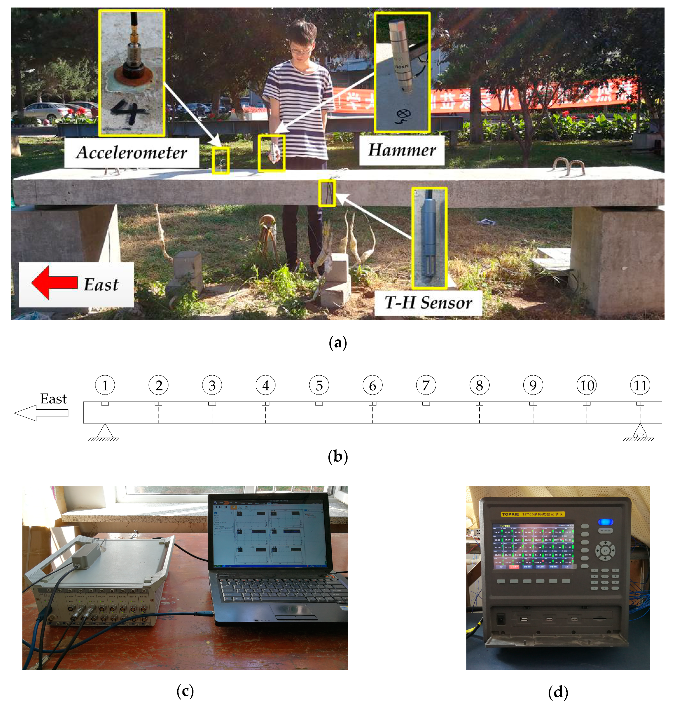
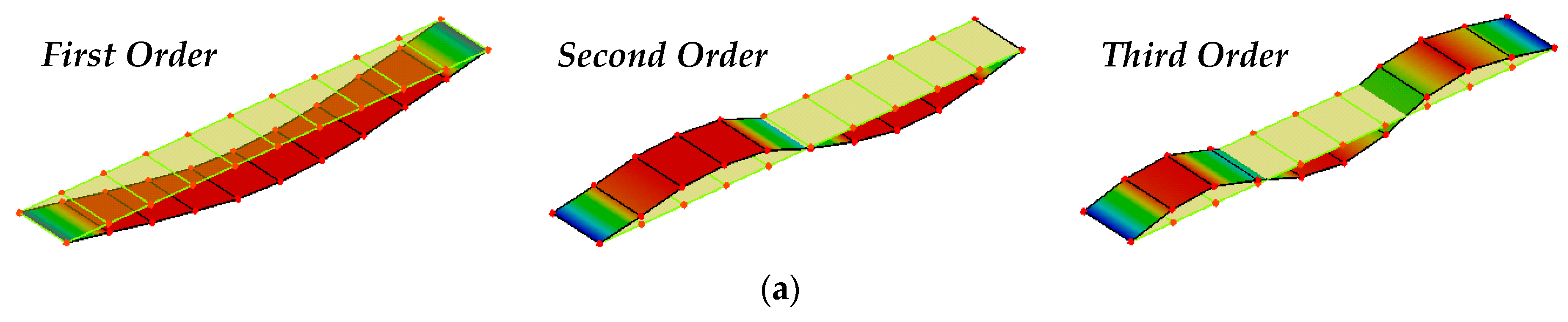
As for the deflection calculated through the dynamic method, we carried out the modal testing with the bridge divided into 11 nodes and 21 nodes, respectively, and extracted the first three vertical vibration modal parameters by the DH5922 type dynamic signal measurement and analysis system.
Figure 7 illustrates the first three vertical MSs analyzed by DHDAS-2013 software platform which is an important part of the DH5922 system.
If the bridge is divided into more nodes, deflections at more nodes can be acquired more preciously. However, the modal analysis with more nodes will make it time-consuming and uneconomically. The proposed deflection calculation method based on modal flexibility and improved Kriging method can solve this problem perfectly, even though MSs with just a few nodes are obtained. Here the mode shapes with 21 nodes are chosen as the benchmark ones, and the ones of 11 elements as the input information are utilized to calculate the mode shapes of 21 elements through the surrogate model. The Kriging method is constructed with regression model and correlation model. The regression models are abbreviated as RM0, RM1, and RM2 for zero, first and second order polynomials in this paper, respectively. Gaussian model has been widely used as a common correlation model due to its good applicability. Besides, the parameter θ in correlation model is another essential part which controls the performance of Kriging model. The Kriging method is implemented in the toolbox DACE of MATLAB [
37].
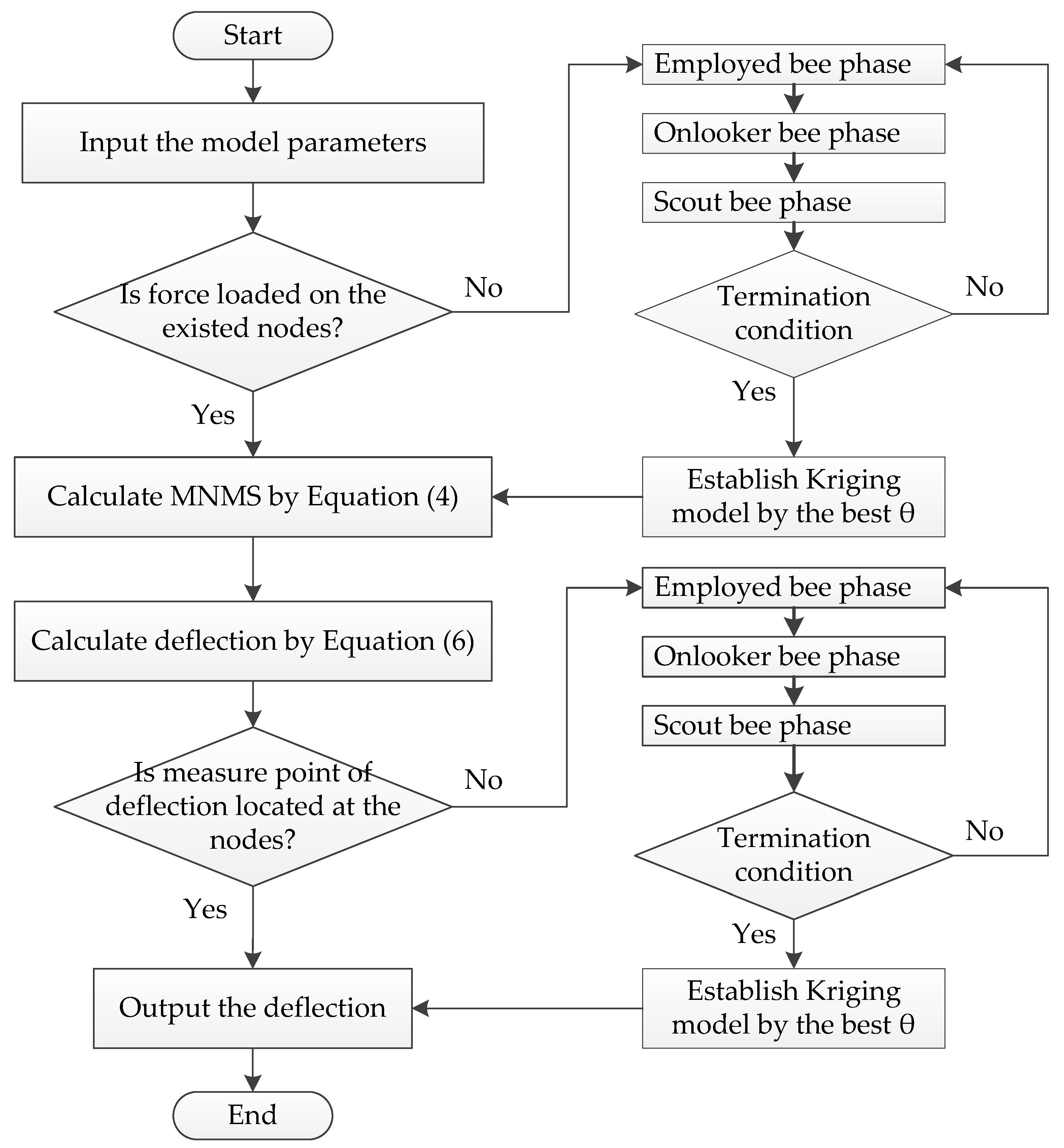
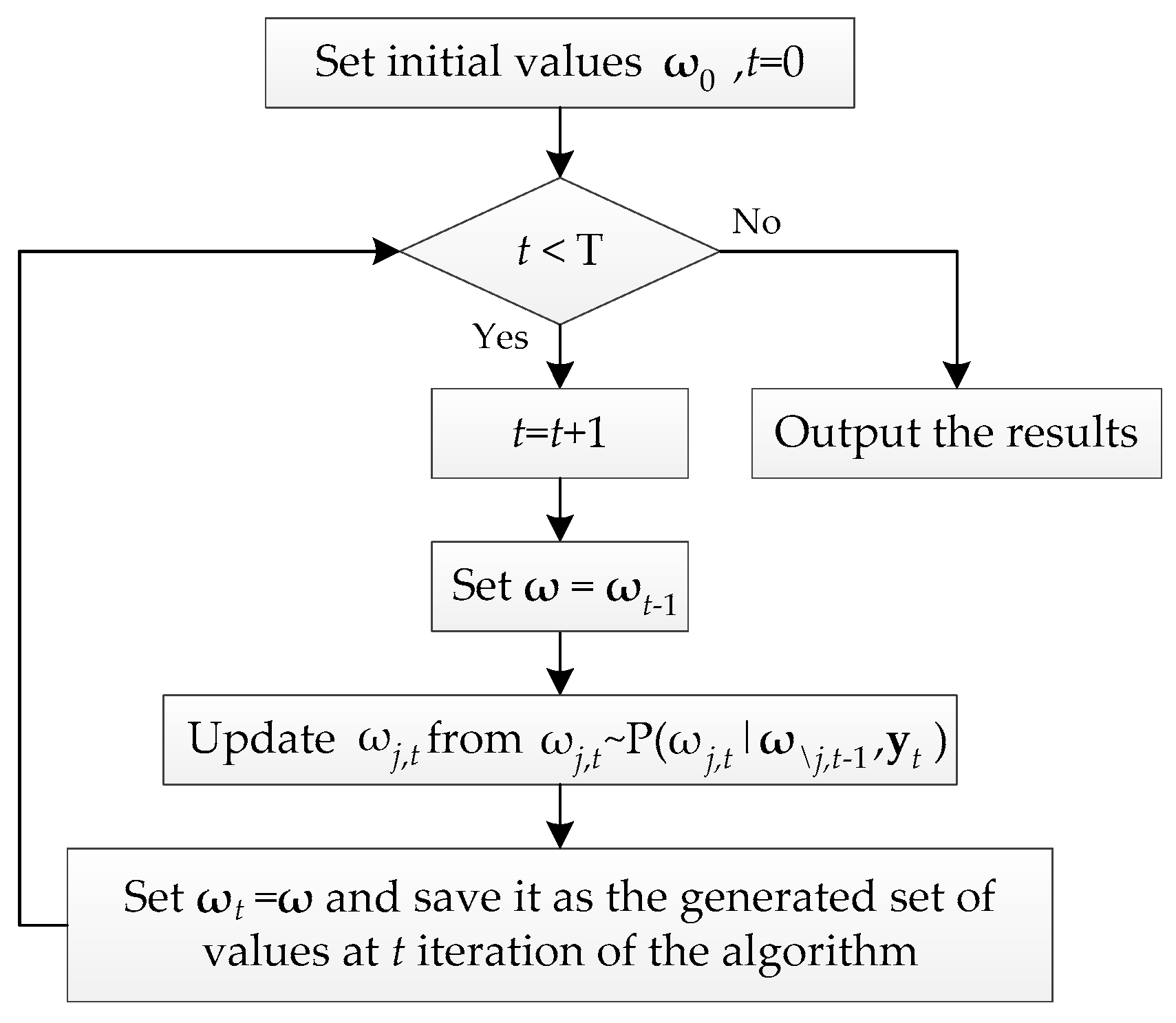
In this article, we establish the optimal surrogate model by the improved Kriging method based on ABC algorithm, of which the particular process has been depicted in
Figure 1. As for the parameter values of ABC, we refer the literatures [
40,
41] and the bee colony size, the control parameter and the maximum number of iterations are set to be 50, 50, and 500, respectively. The object function of ABC algorithm is defined by a Euclidean distance between the
ith order simulated and measured MSs (expressed as Equation (32)), which is also used as an error index to evaluate the fitting quality. It should be noticed that
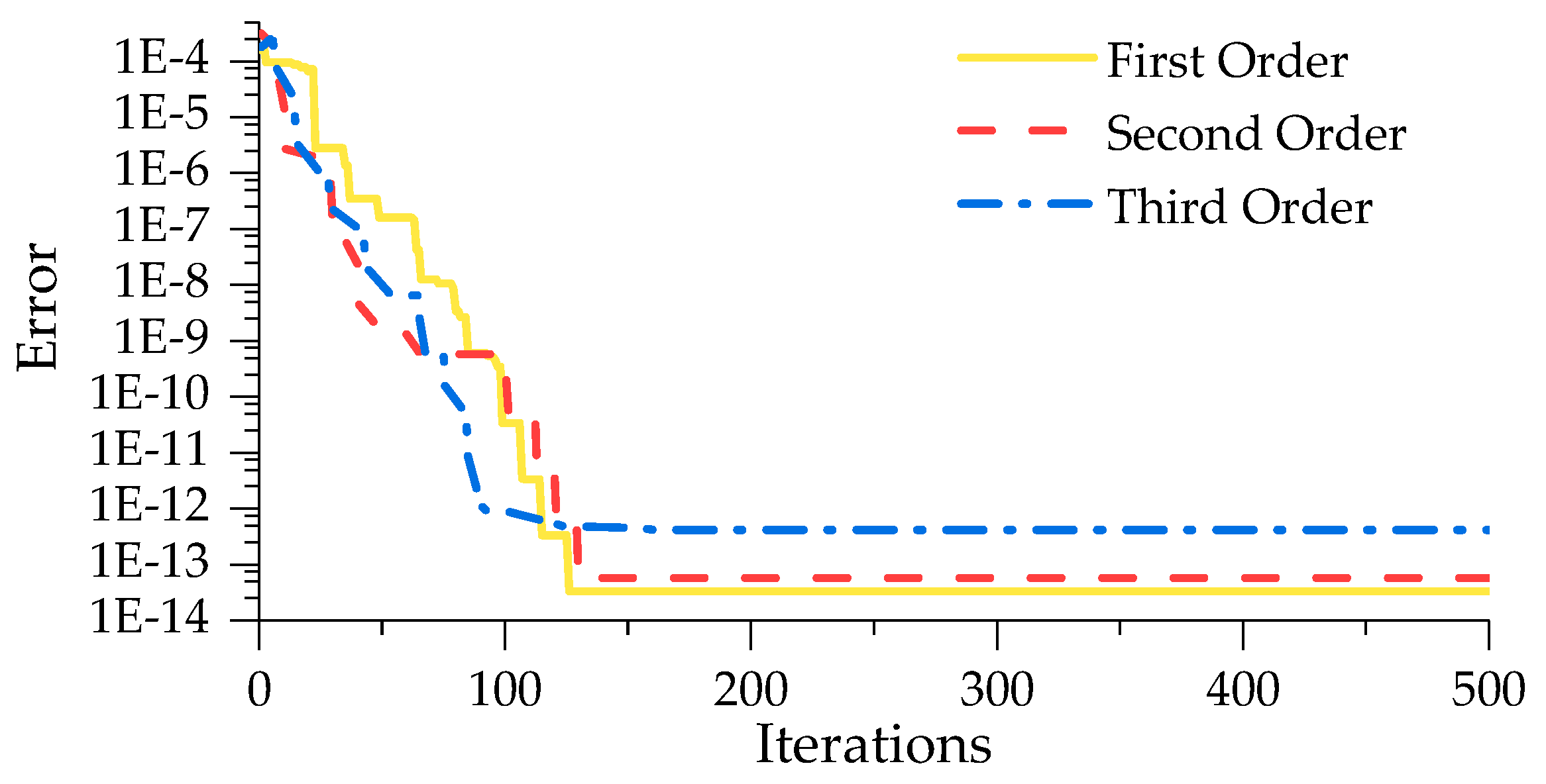
N equals to 11 at this time. The corresponding iteration processes for searching the best θ for the first three modes are shown in
Figure 8. Therefore, we can obtain an improved Kriging model using the best θ. Due to the influence of regression and correlation models, we determine the optimal combination of them with comparing the simulated and measured results depicted in
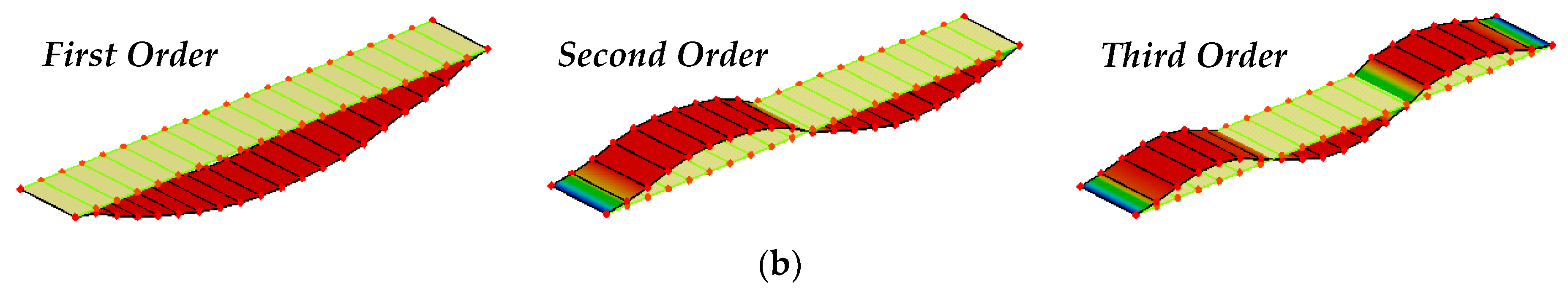
Figure 9 which illustrates the simulated first three vertical MSs with 21 nodes. Once more, the index defined by Equation (32) is employed to estimate the error (described in
Table 3) between the actual measured and simulated MSs with 21 nodes.
where
is the error between the
ith order simulated and measured MSs;
is the
jth node values of the
ith order simulated MS vector while
is that of the actual measured one;
N is the number of nodes.
As can been seen in
Figure 8, ABC algorithm converges at 130 iterations approximately, and the magnitudes of error decreases from 3.15 × 10
−4 to 3.36 × 10
−14. Here, just a typical set of the iteration processes is presented in
Figure 8 and the maximum error for all the iteration process results does not exceed 1 × 10
−12. It demonstrates that the improved surrogate model has favorable applicability and can identify the object MSs accurately. It is a remarkable fact that the Kriging method composed by different combination of regression and correlation models with its corresponding best parameter θ, has sufficient accuracy to fit MSs.
Through the comparison in
Figure 9, we can confirm the surrogate model constructed with the RM0 or RM1 and Gaussian models has the best performance for MSs fitting intuitively. The simulated MSs in
Figure 9b, which are visually same with the actual measured ones in
Figure 9e, are smoother than those in
Figure 9a,c,d. According to
Table 3, the Kriging method based on Gaussian model possesses the smallest error except combining with RM2 for first order MSs, while that based on the exponential model possesses the largest error. As for the method composed by the other two correlation models, its error ranges from 0.3532 to 0.7229, which proves they cannot simulate the MSs precisely. From the perspective of the regression models combined with Gaussian model, the errors caused by RM0 and RM1 are approximate, and RM2 provides larger error. In addition, it is worth mentioning that there is a huge gap between the errors shown in
Figure 9 and
Table 3, which represent the errors between the actual measured MSs with 11 or 21 nodes and the corresponding ones simulated by the Kriging model based on the actual MSs with 11 nodes, respectively. The error in
Figure 9 is caused by the Kriging method, while that in
Table 3 is induced by the error between two testing results besides the method itself. Therefore, this phenomenon demonstrates that the improved Kriging method can simulate the existing testing data precisely and possesses the ability to predict any unknown node values.
In conclusion, the improved Kriging model composed with the RM0 and Gaussian models performs better than the others, and possesses the smallest error (no more than 0.12). Based on the optimal surrogate model, MSs with all external forces located at nodes can be generated, even when there are only a few MS nodes in the dynamic testing results.
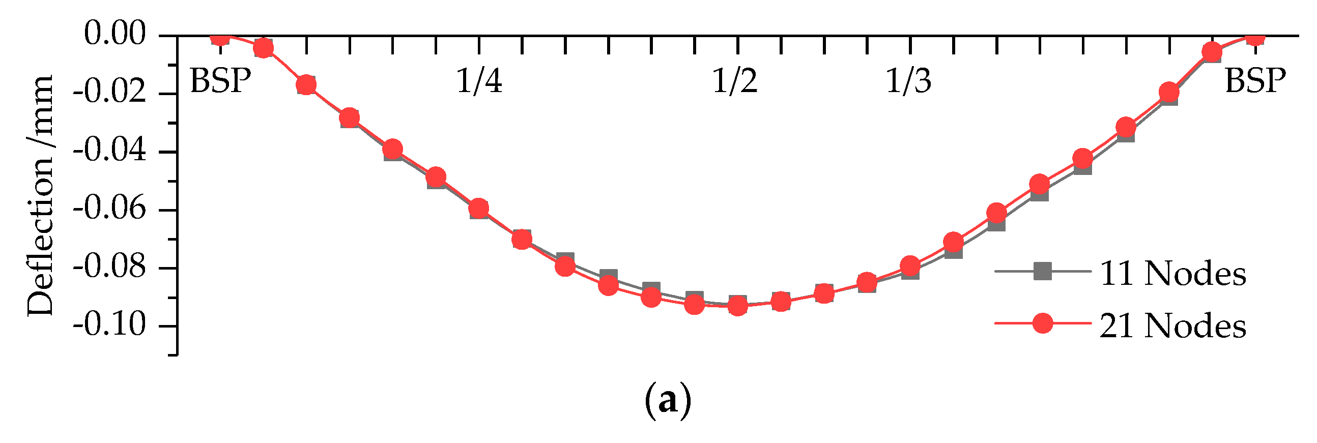
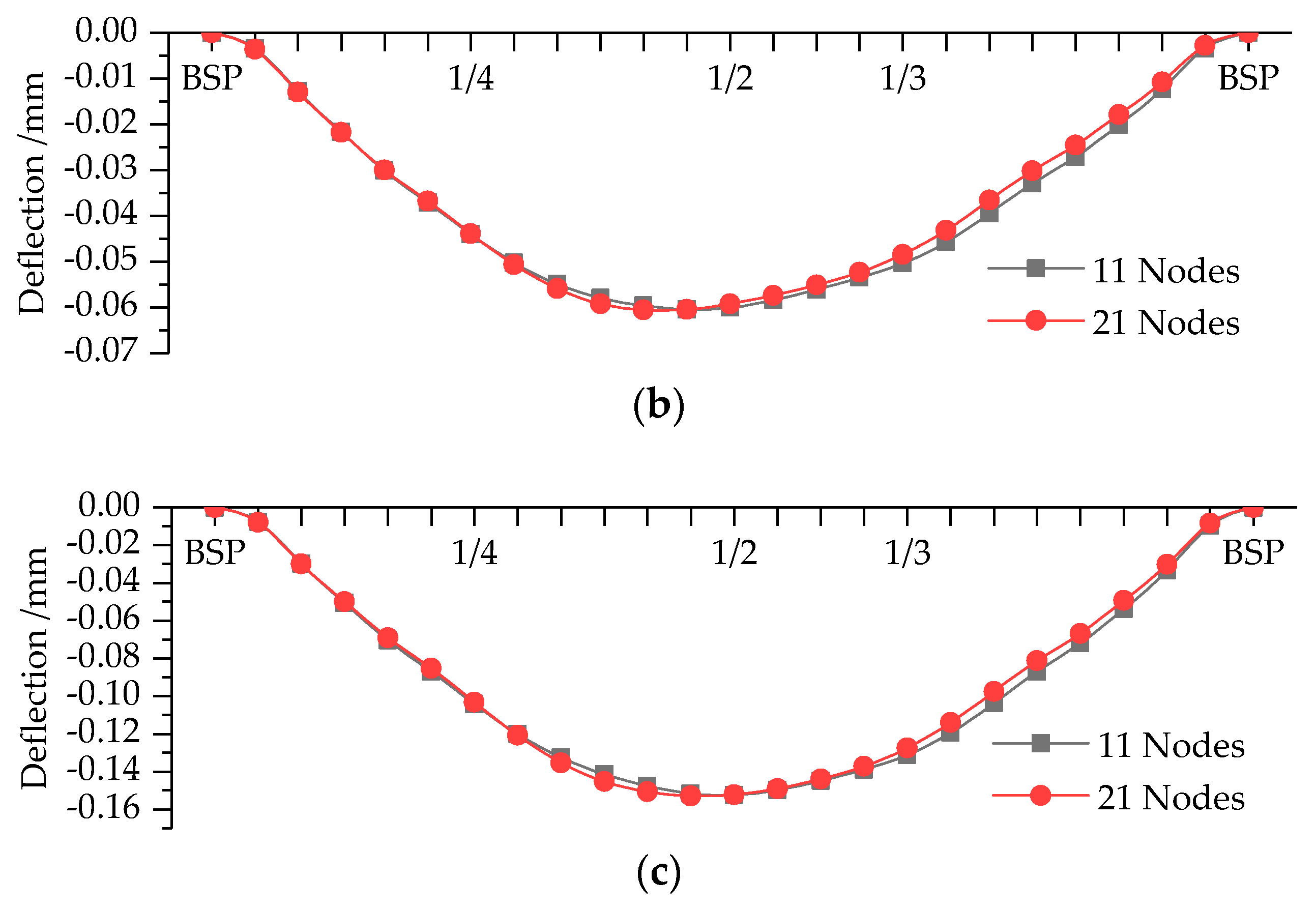
In the second stage of the proposed bridge deflection calculation method, if the deflection of target position cannot be computed through the simulated MSs directly, it will be achieved by employing the improved Kriging method again. Here the method composed with RM0 and Gaussian model also perform the best for this part, and its iteration process for ABC algorithm and the fitting accuracy are similar to the aforementioned results. Bridge deflection curves modeled by Kriging method are depicted in
Figure 10, of which BSP, 1/4, 1/2, and 1/3 represent bridge support point, 1/4-Span, 1/2-Span, and 1/3-Span, respectively.
Table 4 illustrates the particular deflections calculated by the proposed method based on modal flexibility and the improved Kriging method, which are compared with the static results in order to validate the proposed method.
As shown in
Table 4, we also carried out four times dynamic testing for both MSs with 11 and 21 nodes and calculated the deflections at measure points of Cases 1 to 3. The COVs of deflection results are less than 0.0427, which demonstrates the proposed method can compute deflection steadily. There are not obvious differences between the results based on MSs with 11 and 21 nodes. In order to terrify the correctness of the proposed method, we utilize relative error between the mean deflections calculated by static and dynamic method as the assessment index. We can confirm that the absolute values of relative error do not exceed 5% except the results at 1/4-Span of Cases 2 and 3 computed by mode shapes with 11 nodes, and the absolute relative error for 11 nodes are generally lager than those for 21 nodes under the same cases. The reason lies in that the deflections are calculated through the improved Kriging method of two times, which inevitably leads to expand errors. There is a certain difference between the predicted and actual measured MSs as described in
Table 3. In addition, 1/4-Span is close to support point, so the accuracy of testing result will be influenced easily. As for the other measure points, the relative error indicates the proposed method can calculate the deflection successfully. The only drawback of the proposed method is that it cannot precisely compute deflection at measure point which is close to support point. Therefore, we have reasons to believe the proposed method based on modal flexibility and improved Kriging model can calculate the deflection of simply supported bridge correctly and precisely.
In this paper, we only take a simple supported bridge as a research object and verify the correctness and accuracy of the proposed method. However, the proposed method for bridge deflection calculation can also be applicable for other bridge types such as concrete continuous box girder bridge [
19] and irregular bridge. As bridge age increases, bridge damage is inevitable. When bridge structure is damaged, bridge deflection curve will be changed. Modal parameters depend on the state of bridge and modal flexibility has been widely used as an indicator for bridge damage identification. Bridge deflection under damage condition can be calculated by the proposed method in this paper. In other words, bridge damage is another influence factor for deflection calculation. In the future studies, we will investigate and verify the applicability of the proposed bridge deflection calculation method for damaged structure and other bridge types.
5.2. DBN Result Analysis
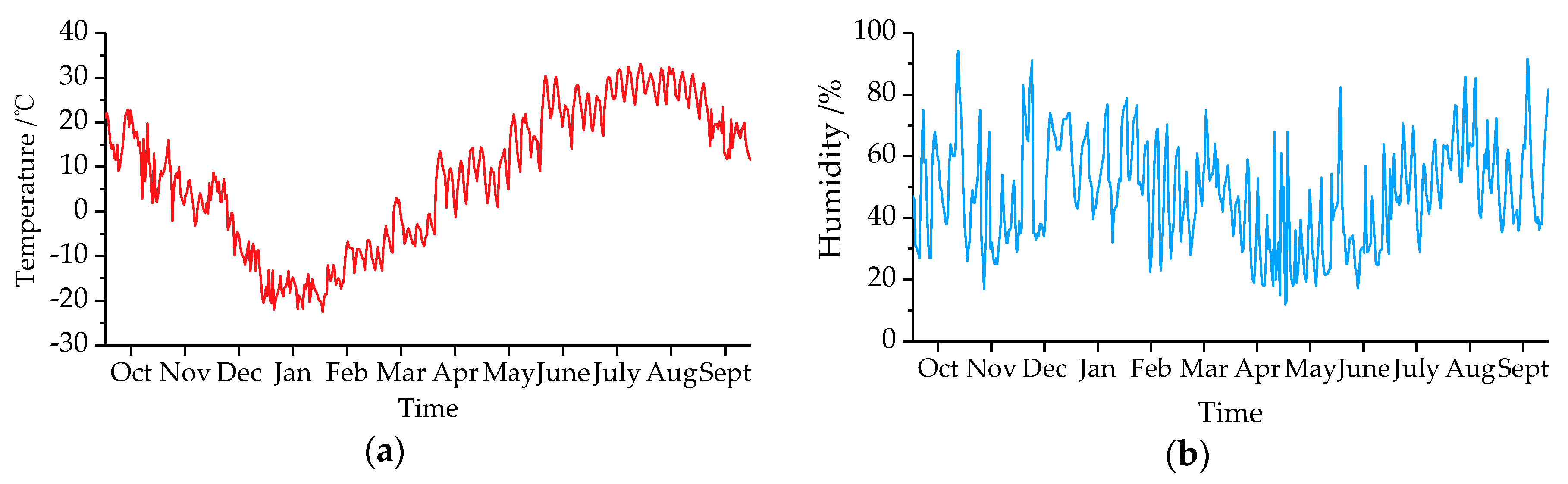
Through the bridge SHM system, the environment temperature and humidity were measured and shown in
Figure 11. It revealed environment temperature of cold region varied widely, which ranged from −22.5 to 32.5 °C affected by an annual cycle. However, no obvious rule for relative humidity variation was observed.
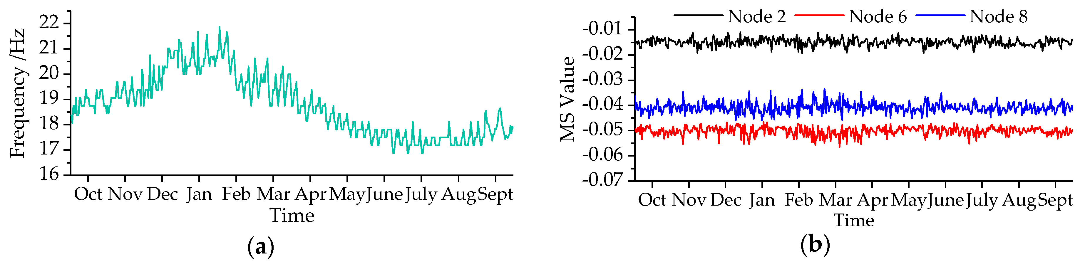
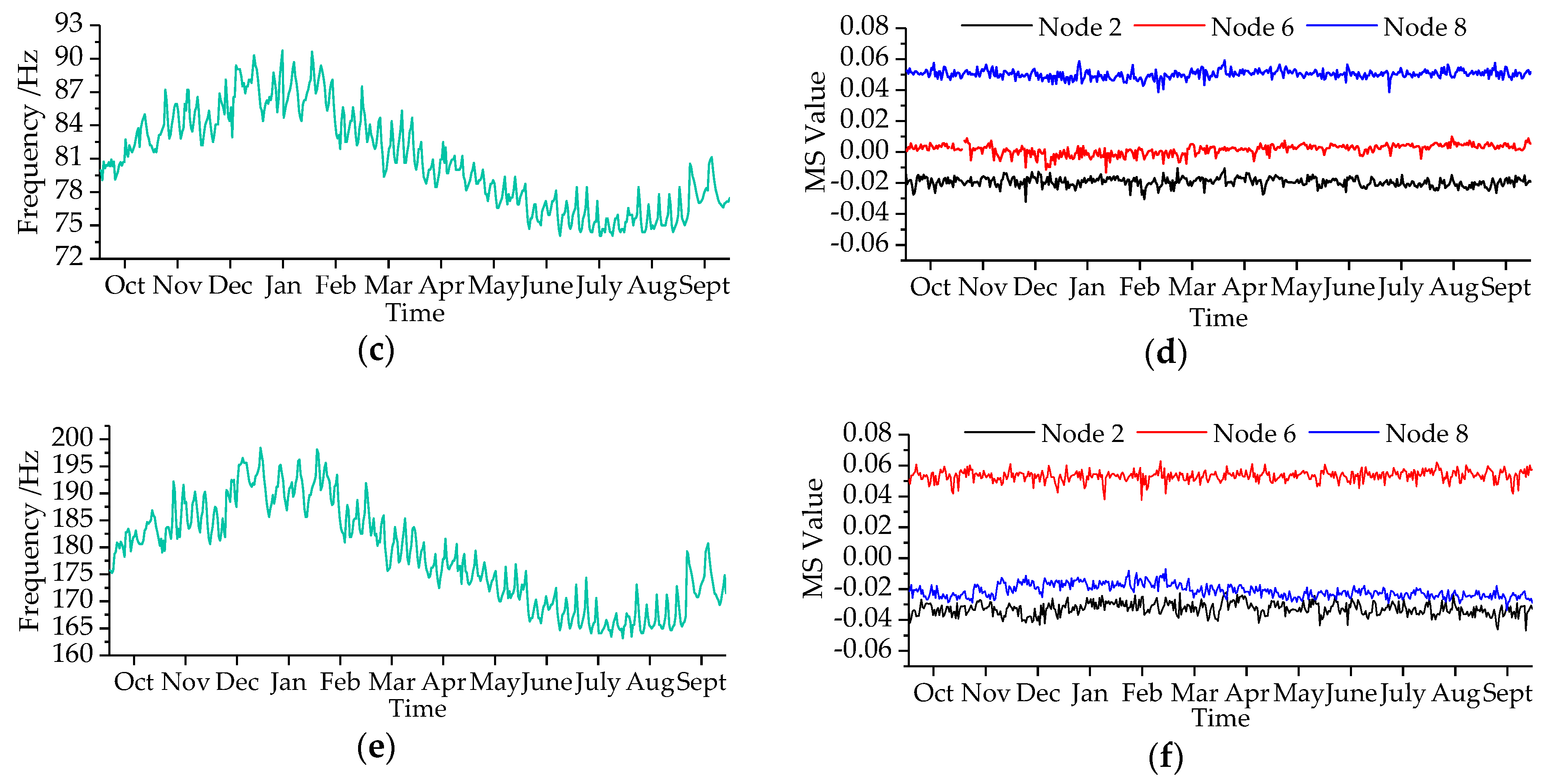
Figure 12 illustrates the variations of the first three modal parameters with time. The first three modal frequencies have opposite trends with temperature variations. In the monitoring process, we identified maximum displacement normalized MS with 11 nodes and transformed it into MNMS by Equation (4). Nodes 2, 6, and 8 were selected as the typical ones to demonstrate the MS value variations, which revealed that there were little changes in the MS.
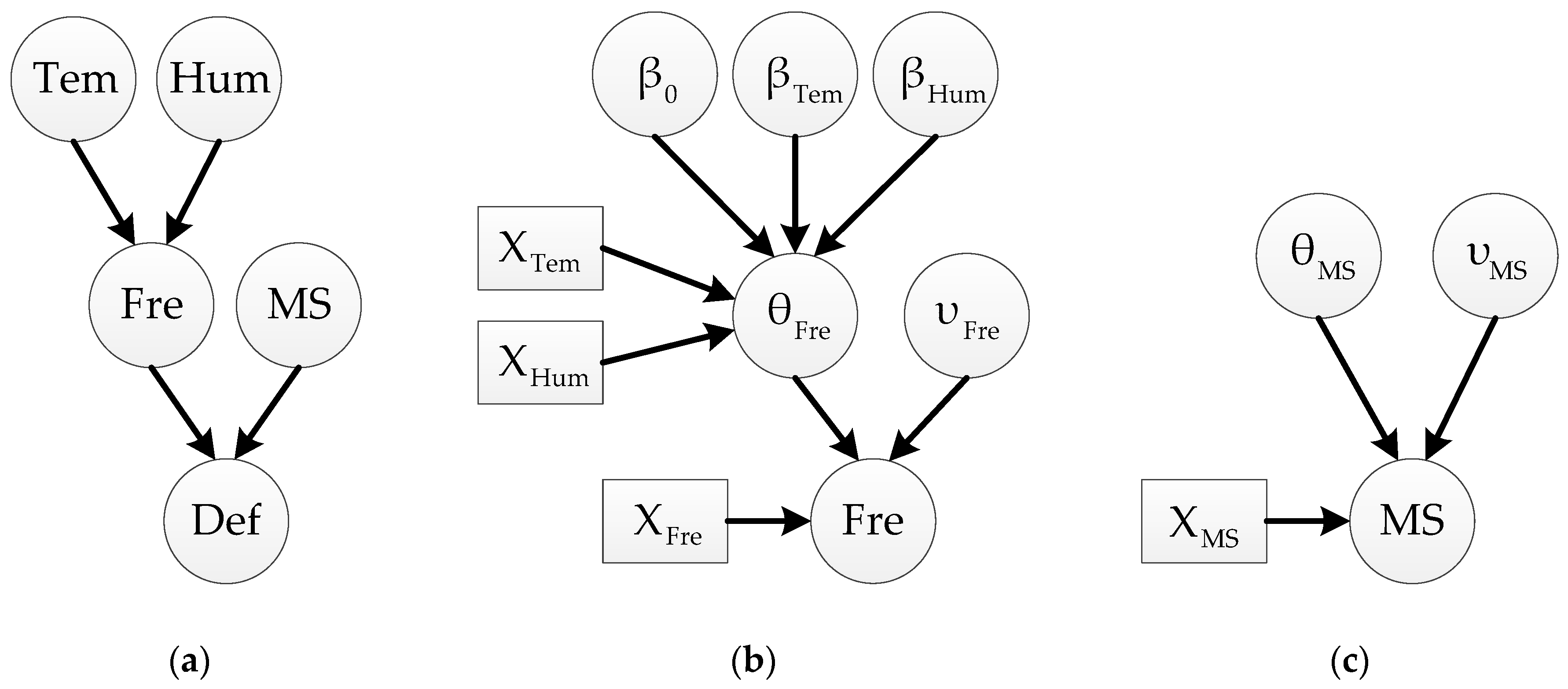
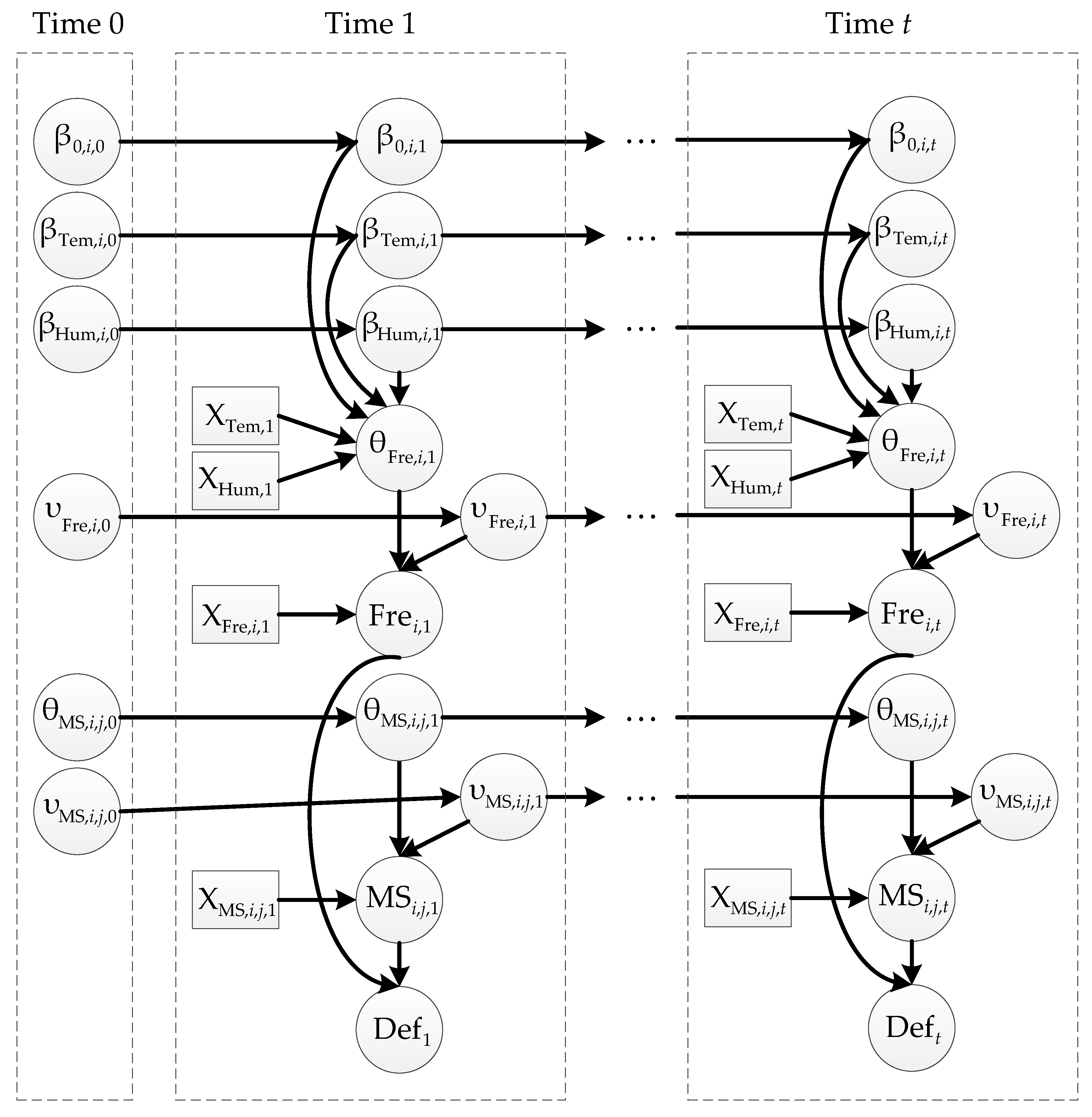
With the observed SHM data, WinBUGS was utilized to analyze the DBN depicted in
Figure 3, of which the iterations were set to be 6000, and the initial 1000 ones were discarded as burn-in. The monitored data in a month was used for a time slice of DBN, namely Time 1 to Time 12 were corresponded with October 2015 to September 2016. In this paper, we assumed the regression coefficient variable β and mean variable θ following normal distribution, and variance variable ν following gamma distribution, because normal and gamma distribution were demonstrated to be appropriate for mean and variance variables in reference [
43]. It should be noticed that if the prior information for Time 1 is unknown, it can be regarded as low-information prior. Therefore, we set prior mean and variance as 0 and 10
4 to represent high uncertainty. A part of posterior summaries of first order in Time 1 are selected as typical results and described in
Table 5.
Here, MC error is used to reflect the estimated accuracy of posterior information. If MC error is lower than 1/20 of its corresponding posterior standard deviation, we can assume DBN converges with high precision. Not limited to the posterior results in
Table 5, all the variables are satisfied with the convergence criteria. Through Kolmogorov–Smirnov test, it demonstrates posterior distribution of variables follow the same probability distribution with their priors. Based on the posterior means, we can end up with regression model of frequency. The regression models for the first three order frequencies at Time 1 are written as
As can be seen from Equations (33)–(35) and
Table 5, it can be inferred that both environment temperature and humidity have important effects on modal frequencies. For every increase of the temperature by 1 °C, the decrease of first modal frequency at Time 1 lies between 0.03546 Hz and 0.02273 Hz with probability 95%. This phenomenon is consistent with the conclusion in reference [
29]. When humidity increases 1%, the frequency is expected to decrease 0.006749 Hz averagely. According to modal frequency calculation formula of simply supported bridge, modal frequency will decrease when bridge mass increase. The increase of humidity may cause a little of increase of bridge mass, so it coincides with the modal theory. With mode order increasing, modal frequency values will be influenced by these two environment factors more obviously. The variation intervals of the third modal frequency even reach up to 0.3493 Hz and 0.0535 Hz on average for unit change of temperature and humidity, respectively. Considering another perspective, it also demonstrates that humidity has much less contribution on modal frequency variations than temperature. The total variations of the first three modal frequencies influenced by humidity are 0.493 Hz, 1.67 Hz, and 3.91 Hz. They are all lager than the frequency resolution, which illustrates the observed influence of humidity is not caused by measurement noise. The standard deviations of all variables are so small that the posterior distributions of modal frequencies and MSs can be predicted precisely through the posterior parameters shown in
Table 5. The variables not listed in
Table 5 have the same variation trends and rules. In addition, it should be noticed that the test environment belongs to cold region, which means the results only can be referred for bridges in cold region. However, the proposed method can be used for any kind of environments.
5.3. Dynamic Reliability Analysis of Simply Supported Bridge Deflection
As described in the sections mentioned above, we proposed the simply supported bridge deflection calculation method and elaborated the DBN analysis process for probability distributions of relative modal parameters. According to the standard requirements of design code [
49], maximum deflection value, which generally locates at 1/2 span of bridge, cannot be more than 1/250 of its span length
l when
l is less 7 m. Hence, the performance function for simply supported bridge deflection can be defined as Equation (36), in which the parameter meanings are identical to those of Equations (5) and (6).
The corresponding failure probability (FP) and reliability index (RI) can be defined as
where
represents the inverse standard normal cumulative distribution function.
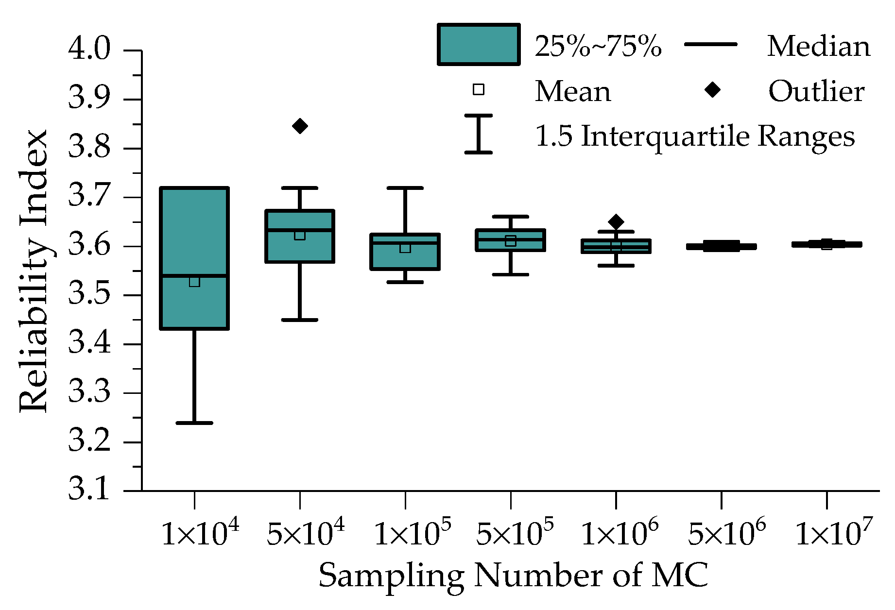
In this paper, the performance function is calculated based on modal flexibility and Kriging method, which is difficult to obtain the closed-form solution of Equation (37). So Monte Carlo (MC) simulation method is employed to solve this problem. MC method possesses the best performance in calculation accuracy and applicability except computation time, which increases with the sampling number. Based on DBN analysis results of the variables probability distribution, we take the RI calculation process of Case 1 in January 2016 with 20 kN external force as an example. The sampling numbers are set to be 1 × 10
4, 5 × 10
4, 1 × 10
5, 5 × 10
5, 1 × 10
6, 5 × 10
6, and 1 × 10
7, and it is computed twenty times for each sampling number. The boxplot of computation results is depicted in
Figure 13. With sampling number increasing, the dispersion of RI results decreases gradually, and it converges when the sampling number exceeds 1 × 10
6. The computation time of MC method with sampling number 5 × 10
6 is less than 2 min, while that for 1 × 10
7 is even more than 15 min. The former is within the acceptable range, so the sampling number for MC method is set to be 5 × 10
6 in the following computations.
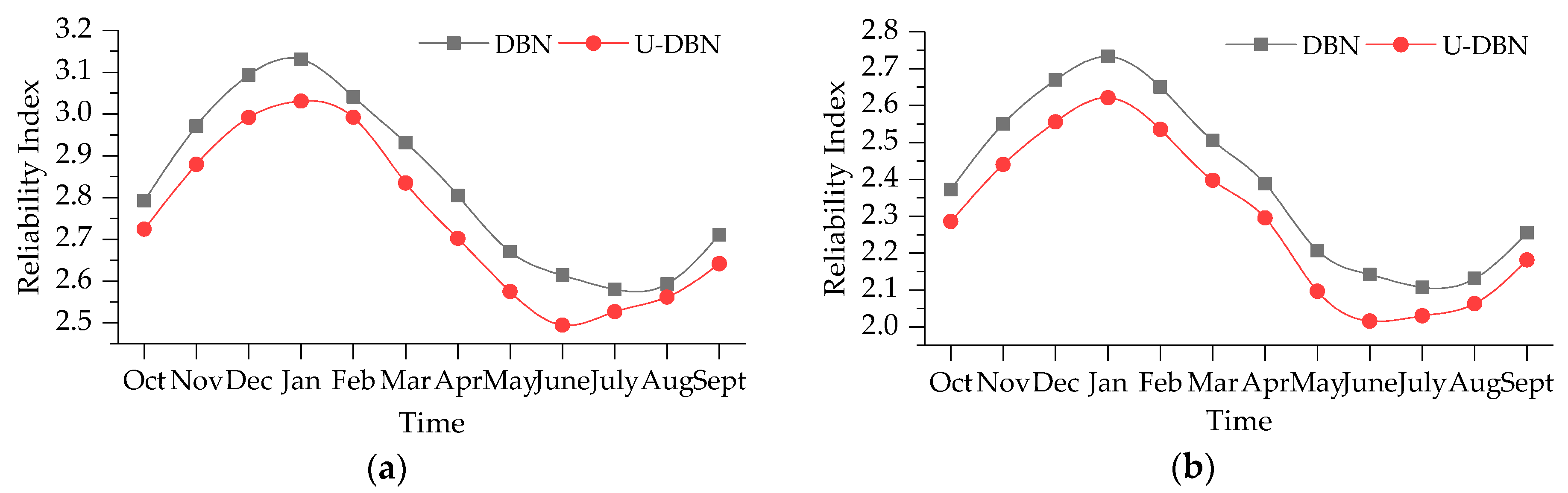
In order to analyze the dynamic reliability of simply supported bridge, we calculated the reliabilities of Case 1 and Case 3 mentioned above, respectively. The external forces for these two cases are both assumed lognormal distributed with mean 15 kN and standard deviation 6 kN. The time-dependent reliabilities based on DBN method are shown in
Figure 14. They are compared with that calculated through the probability distribution (U-DBN), which are identified by the monitoring data from October 2015 to September 2016.
In
Figure 14, it is shown that the time-dependent reliability is negatively correlated with environment temperature (shown in
Figure 11a). The maximum RIs of Cases 1 and 3 calculated by DBN method are 3.13 and 2.73, while the minimum ones are 2.58 and 2.11. For Cases 1 and 3, the minimum RIs decreases by 17.6% and 22.7% compared with the maximum ones. The maximum and minimum RIs are corresponding to January and July, which have the lowest and highest temperature, respectively. We can also confirm that the RIs calculated through U-DBN are all lower than the results of DBN, namely it underestimates the bridge deflection reliability. According to the correlation between the reliability and temperature, the lowest RI should occur in July; however, the lowest RI calculated by U-DBN occurs in June in
Figure 14. It demonstrates the proposed bridge deflection reliability calculation method based on DBN can reduce the influence of uncertainty and improve the reliability assessment accuracy.
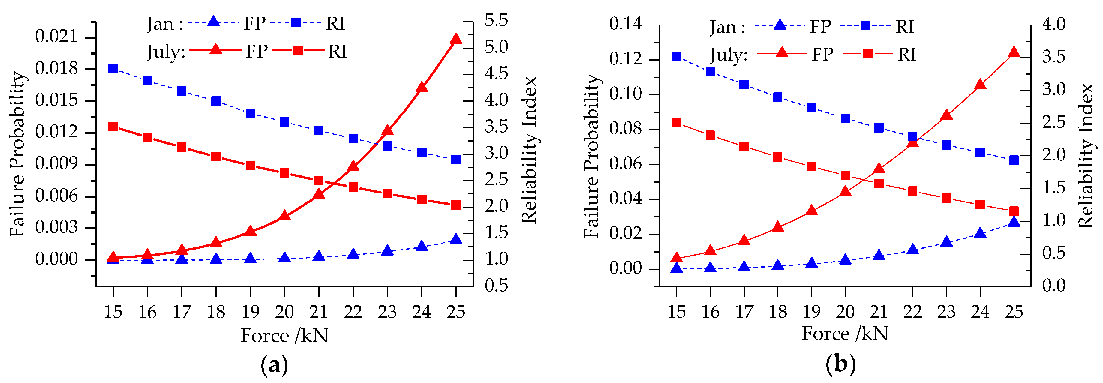
Figure 15 depicts the bridge deflection FPs and RIs of January and July with external forces from 15 to 25 kN. The RIs of January range from 4.61 to 2.90 for Case 1 and from 3.52 to 2.04 for Case 3, while those of July range from 3.52 to 1.93 for Case 1 and from 2.50 to 1.16 for Case 3. The FP curves present exponential with external force increasing. RI can be utilized to determine vehicle load limitation of actual bridge. In actual engineering, vehicle load limitation is set according to ultimate limit states of bridge without considering environment influence and structural health monitoring, and it seems to be not safe or accurate enough. However, it can be provided reasonably through the reliability calculation method proposed in this paper. For example, if the target RI is set as 3.0, the external force should be limited lower than 17 kN for Case 1.
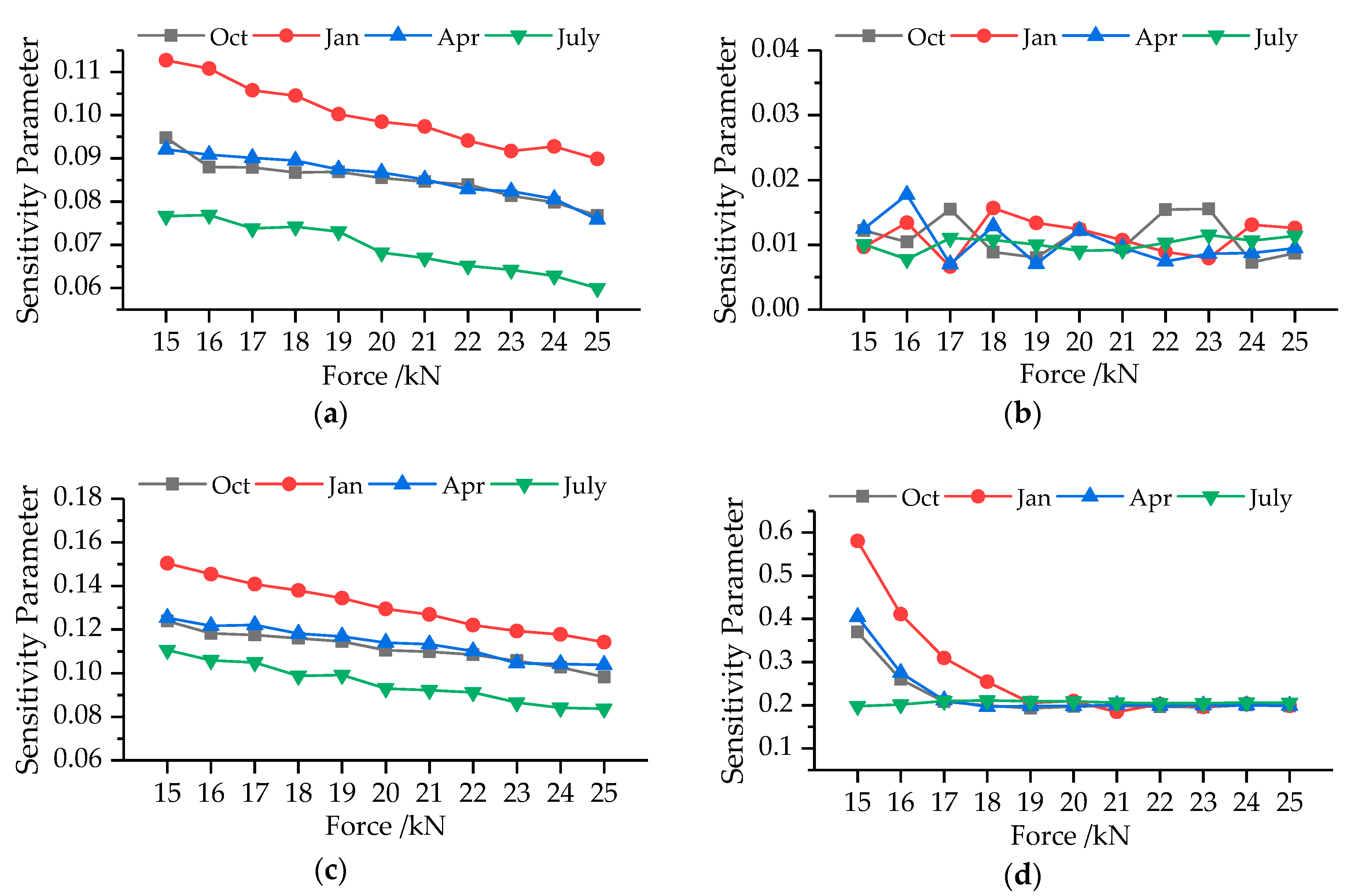
5.4. Sensitivity Analysis of the Variables
In this work, we computed the dynamic RIs combining with the modal parameters and environment factors. To investigate the effect of influence factors on the RI results, a quantitative sensitivity parameter introduced in reference [
50] is employed here (defined as Equation (39)). The RI sensitivity results of modal frequency, MS, temperature and humidity in October 2015, and January, April, and July 2016 for Case 1 are shown in
Figure 16.
where
represents the quantitative sensitivity parameter;
is the original reliability index mentioned above;
is the reliability index calculated without considering one of the influence factors (IF), namely it is taken as a constant while other factors are maintained as statistical variables.
As can be seen from
Figure 16, environment temperature, modal frequencies and MSs are major parameters affecting the bridge deflection RI. The SP of environment humidity is approximately 0.01 and ranges between 0.05 and 0.02 irregularly, which reveals humidity has little influence on bridge deflection RI. As for temperature and frequencies, the SP decreases linearly with force increasing, which demonstrates these two factors play less important roles in the RIs when external forces become larger. In
Figure 16a,c, the SP in January possesses the largest value while that in July is the smallest under the same condition. SP in April is slightly larger than that in October in most conditions. This phenomenon illustrates that temperature and frequencies have more important effects on bridge deflection RI in low temperature environment. In addition, the largest and smallest values in
Figure 16a are 0.113 and 0.059, and those in
Figure 16c are 0.151 and 0.084. Modal frequency makes more contribution on bridge deflection RI than temperature. In the SP curves for MS, there is a critical force value. The SP decreases with force increasing when external force is smaller than the critical force value and becomes a constant when external force is larger than the critical force value. The critical force value becomes larger as the environment temperature decreases. Because temperatures in April and October are similar, the SP curves have the same variation tendency. The largest SPs of MS are 0.581, 0.405, 0.369 and 0.211 in January, April, October, and July, while the smallest one is about 0.2 for all of them. Therefore, the bridge deflection RI is more sensitive to MS than the other three factors.


