2D Triangulation of Signals Source by Pole-Polar Geometric Models


Abstract
:1. Introduction
1.1. Considerations about Signal Data
- and are the receiver and the emitter power
- and are the receiver and emitter antennas gains
- is the radial distance between an emitter and a receiver in meters.
- is the wavelength. For IEEE 802.11b and g to 2.4 GHz, and, to 5.7 GHz, .
1.2. Standard Methods and Considerations
1.2.1. RSSI Approach
- is the signal strength value (dB) expected by an AP located at a radial distance
- from the signal origin.
- is the signal strength value (dB) at some reference distance .
- indicates the rate at which the path loss increases with distance (empirical value).
- is the signal attenuation factor promoted by walls.
- is the signal wavelength.
- is a Gaussian noise with zero-mean and variance .
1.2.2. Time-Based Approaches (ToA and TDoA)
1.2.3. Generalization of 2D Location Function Range-Based
1.2.4. How to Solve the System
- ;
- ; ; ; ; ;
- ; ; .
1.3. Useful 2D Geometric Definitions
- (d-1)
- The Euclidean distance between two points and is given by
- (d-2)
- For constants , , ( and not both zero) all points satisfying the equationdefine the implicit line equation in the Cartesian plane. For two points and , a particular line equation is obtained by
- (d-3)
- Two particular lines and have an interception at the point , if , given byif , lines are perpendicular. If , lines are parallel or coincident.
- (d-4)
- The angle formed between two particular lines is given by
- (d-5)
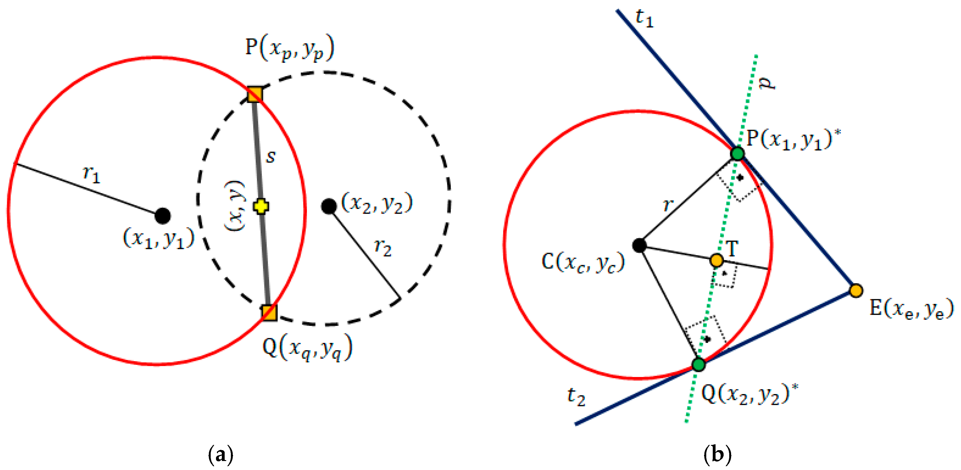
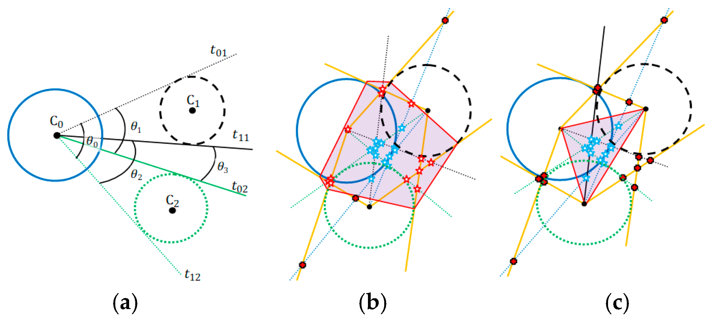
- The line equation that passes through point and is perpendicular to the line is defined asCircle—In the Cartesian plane the equation defines the implicit circle equation centered at the point with radius . Let be an external point to a circle. By using we can obtain two tangent lines, and , to the circle (Figure 1b), which pass through points and , respectively. Points and can be computed by applying the geometric concept of pole-polar definition.Pole-Polar Geometry—Pole-point and polar-line are, respectively, a point and a line that have a unique reciprocal relationship with respect to a given conic section. If the point lies on the conic section, its polar-line is the tangent line to the conic section at that point [24]. If the pole-point is external to the conic section, the polar-line intercepts the conic section exactly at the points that allow passing tangent lines from this pole-point (Figure 1b). Our interest is to pass two tangent lines, and , through a circle centered at point with radius . Moreover, these lines must pass through a known external point (or pole-point) to this circle (Figure 1b). We need to locate the coordinates of the polar-points and , which define the polar-line and lies to the tangents lines and . Additionally we must find the equation of the polar-line .
- (d-6)
- The general equation of a conic in the Cartesian coordinate system is given by . We need the equation of the polar-line that can be obtained by a known pole-point . The required coefficients of the respective polar-line is given by: ; ; . In this work, the expected conic section is a circle. For the circle case, the following simplifications are helpful: ; ; ; ; and .The next step consists in placing points and , which are obtained by computing the intersection between the polar-line and the circle line (Figure 1b). To compute the intersection of a line, , with a circle, , the following conditions must be considered: is the distance between the line and the circle center point ,
- ○
- if , there is no intersection point;
- ○
- if , the line is tangent to the circle and has one intersection point;
- ○
- if , the line is secant to the circle and has two intersection points.
The algebraic solution for this intersection is an equation of degree two. Another way to solve this intersection is applying some geometric relationships, as follows. To find the intersections points and , which are the polar-points, we have first to drop a perpendicular line (by d-5) from the center of the circle to the line . Let be the intersection point and be the line that passes through and (Figure 1b).The equation of line is known (by d-6). Thus, the equation of line is . This way, the point can be computed by intersection between and lines (by d-3).represents the Euclidean distance between points and ; refers to the distance between points and ; stands for the distance between points and ; and (by d-1).The triangles and are right-angled, and hence we prove thatand - (d-7)
- So, ; now, if we translate the point by units in both directions along line , the points and are determined as followsand, ifThe suggested geometric models that use the convex hull algorithm (CHC, PLI, TLI, and MAI) need to minimize the region of interest (ROI) and exclude bad points from final results. This minimization of ROI is obtained by obtaining a convex polygon defined on a set of previously computed points. A set is convex if . Any region (polygon) with a “dent” is not convex [24]. The convex hull of a set of points is the smallest convex set containing these points [24,25,26].
- (d-8)
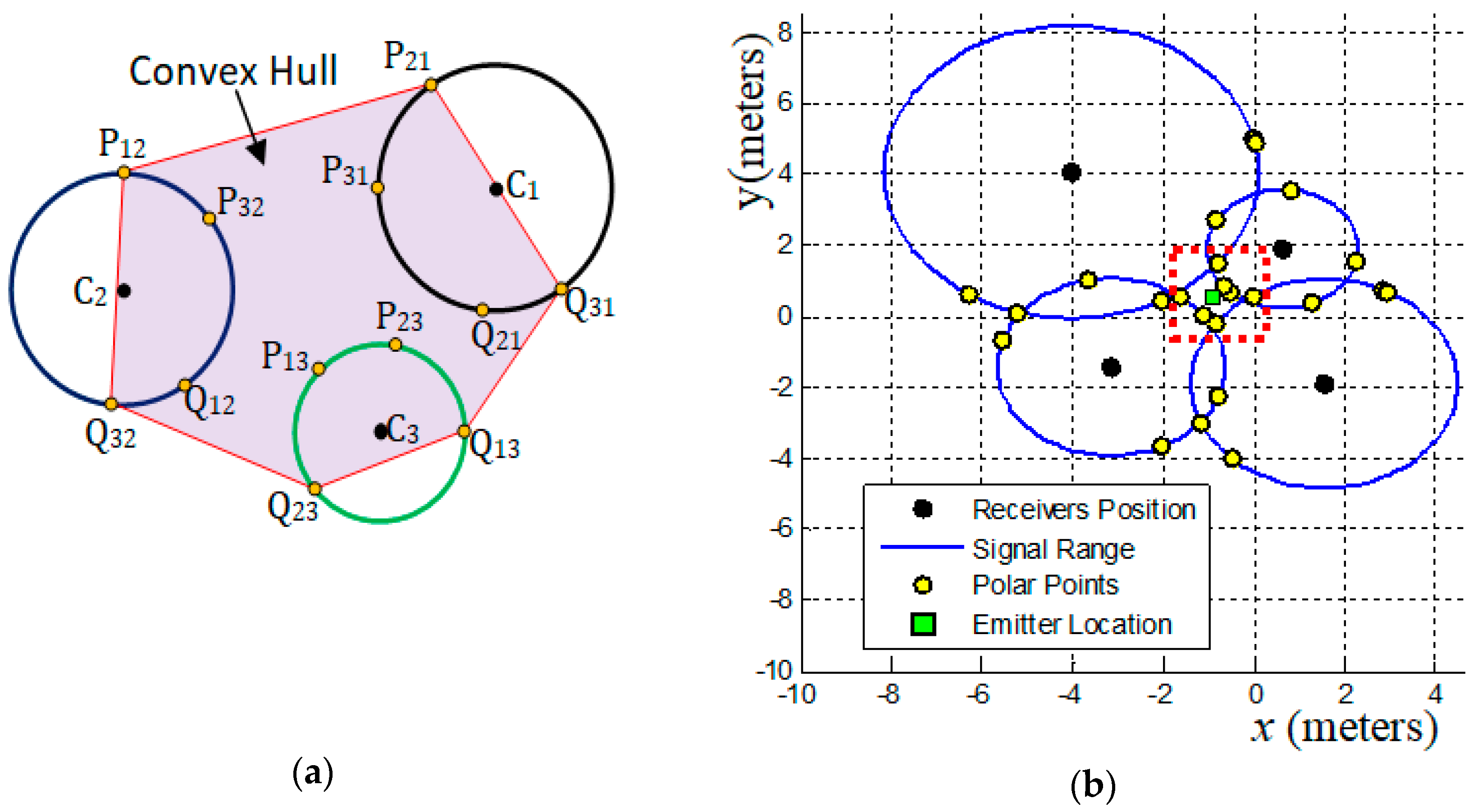
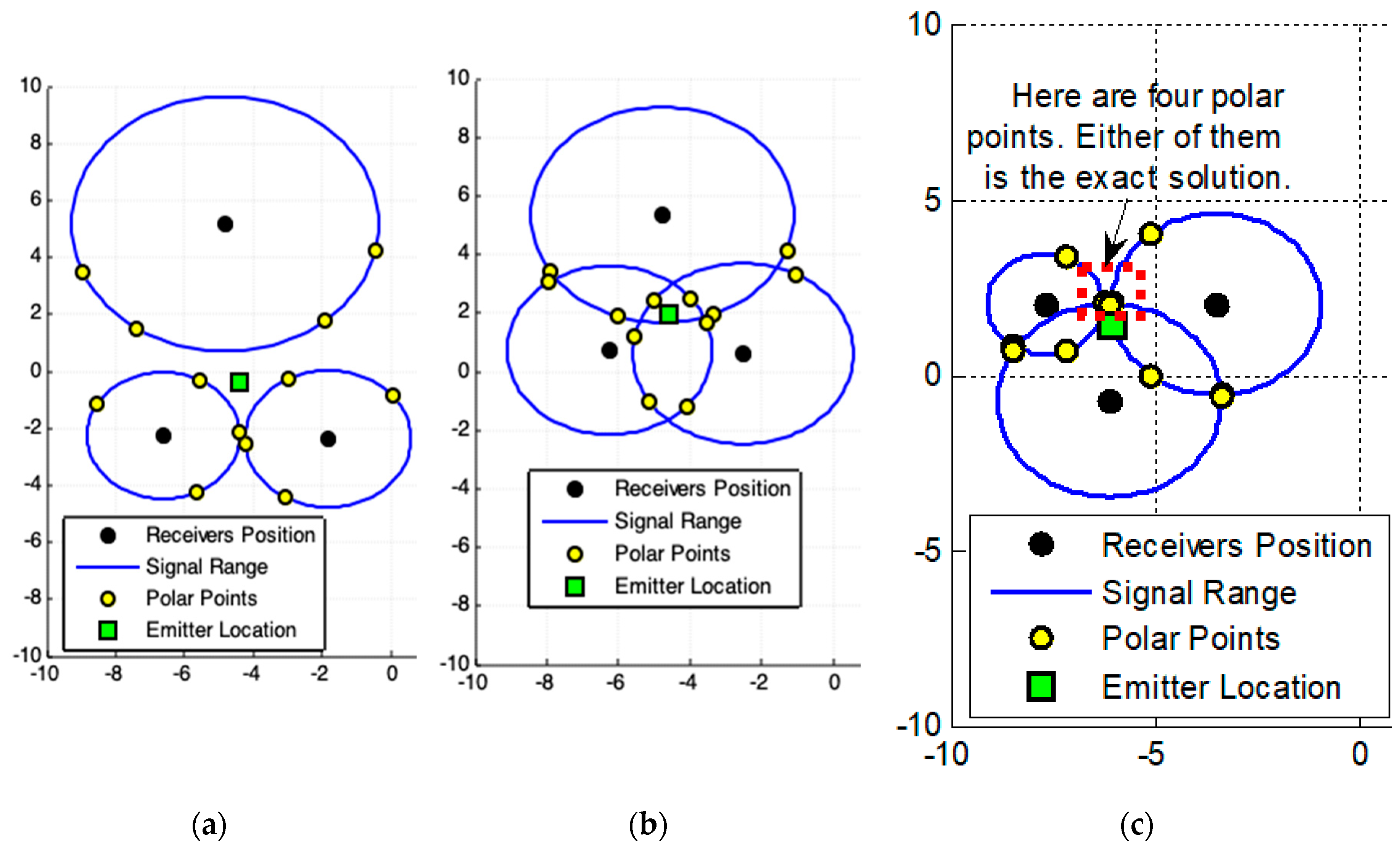
- The convex hull algorithm is used in this work to specify a Region of Interest (ROI).To illustrate the use of the convex hull we must consider the existence of three receivers centered at coordinates (and these coordinates cannot all be collinear) that collect a signal from a point with distance and (radial distance), respectively. and , , represents the polar-points that lie to the circle centered in that is obtained by the external point (center of another circle), as Figure 2a shows. Thus, the smallest convex polygon that contains all obtained polar-points is the convex hull for these points and this minimal polygon defines our ROI. This region in red-color lines is used to illustrate the ROI for the proposed geometric models presented below (always representing a convex hull to define a ROI).
- (d-9)
- The location estimation of the emitter, , is based on a set that contains points, , which are collected in a defined ROI. This location is given by the centroid point among all points in , by
2. The Proposed Geometric Models
2.1. Accurate Data, Exact Result
2.2. Polar-Points Centroid Model (PPC)
| Algorithm 1. PPC—Polar-Points Centroid Model |
| Data Input |
| is the number of receivers. , , is the planar position of each receiver. , is the signal range of each receiver to an emitter. |
| Procedure |
| 1: for each |
| 2: , by (d-6) and (d-7), for each receiver position , used as pole-points, compute all combinations of polar-points and with the respective receiver at position and signal range . |
| 3: store the points and in the set . |
| 4: end for |
| 5: Apply (d-9) in the set , compute the location estimation, , of the emitter. |
| Information Output |
| 6: Emitter location estimation . |
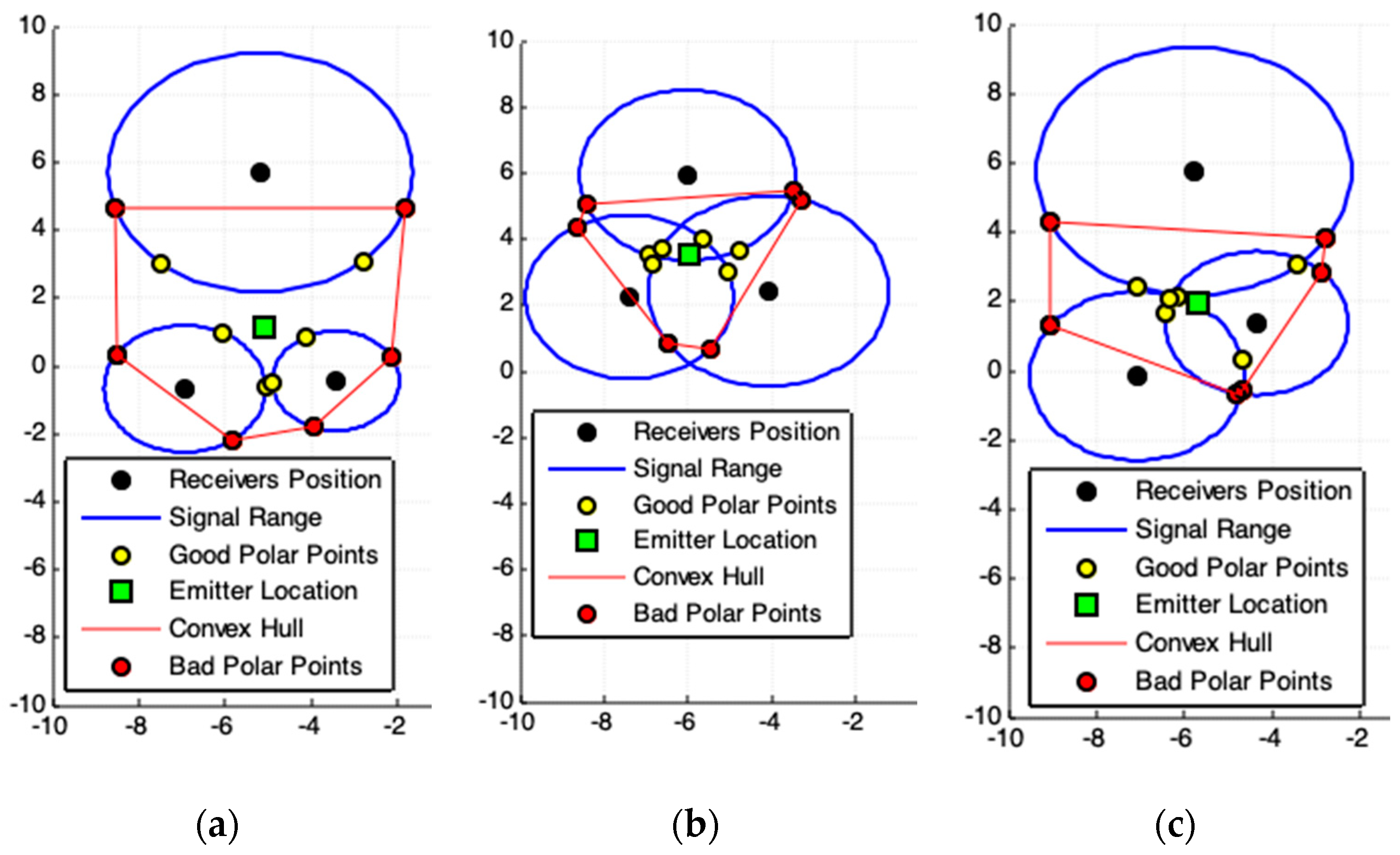
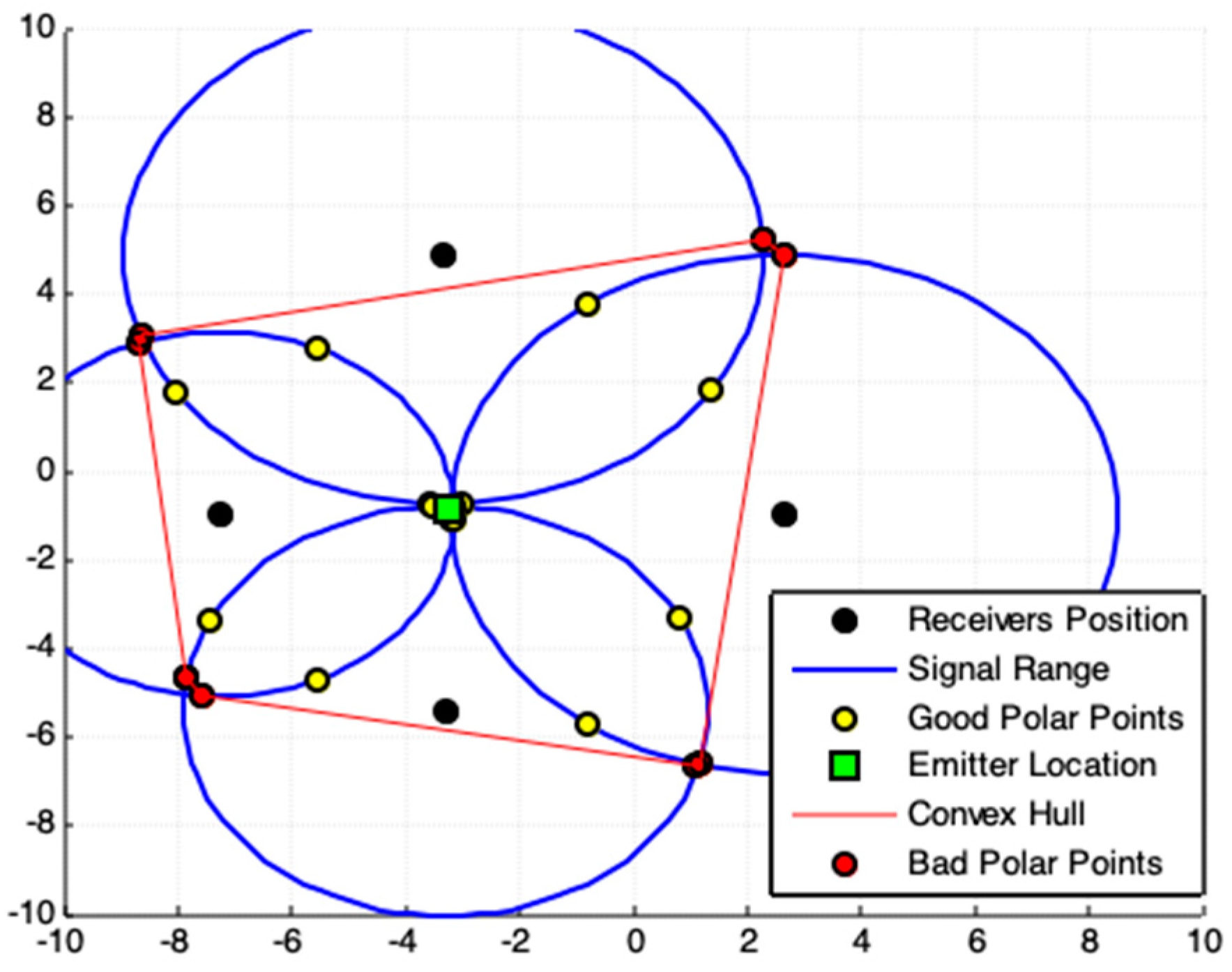
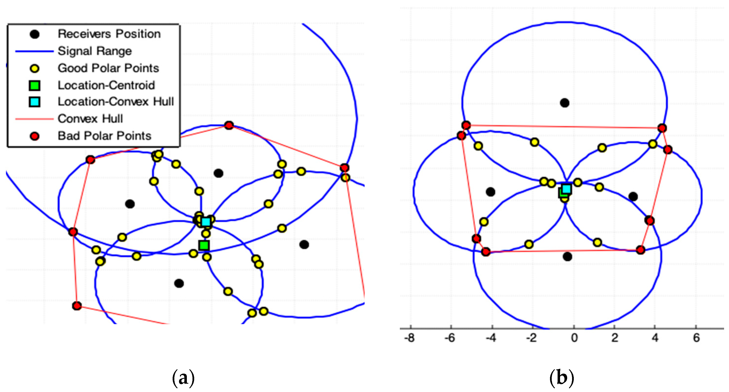
2.3. Convex Hull Centroid Model (CHC)
| Algorithm 2. CHC—Convex Hull Centroid Model Algorithm |
| Data Input |
| is the number of receivers. , , is the planar position of each receiver. , is the signal range of each receiver to an emitter. |
| Procedure |
| 1: Execute the steps 1 until 4 of algorithm Polar Points Centroid Model. |
| 2: Apply (d-8), find the convex hull polygon for all polar-points in . The obtained polygon is the minimal convex polygon that involves all interest points in . This polygon constitutes the ROI. |
| 3: Exclude all polar-points on the boundary of this convex polygon, called bad polar-points, from . |
| 4: Apply (d-9) in , compute the location estimation, , of the emitter. |
| Information Output |
| 5: Emitter location estimation . |
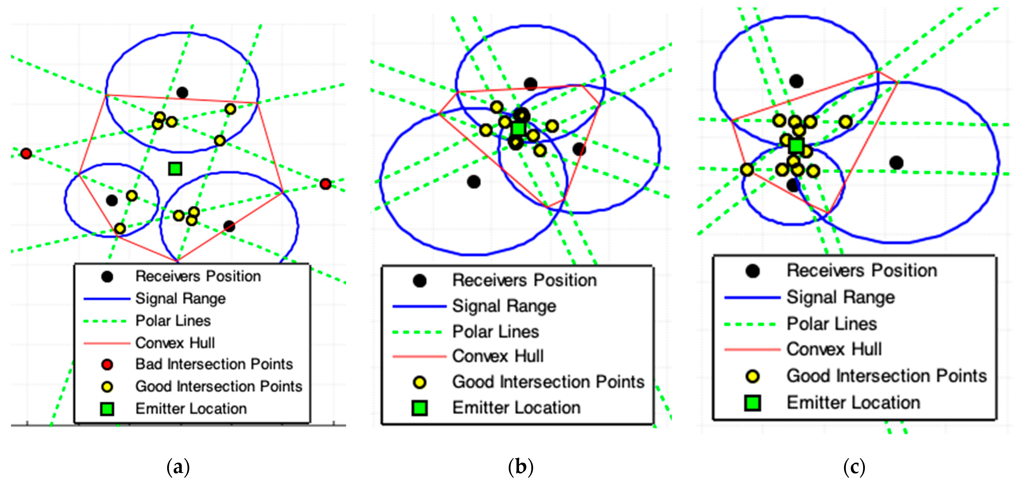
2.4. Polar Lines Intersections Model (PLI)
| Algorithm 3. PLI—Polar Lines Intersections Model Algorithm |
| Data Input |
| is the number of receivers. , , is the planar position of each receiver. , is the signal range of each receiver to an emitter. |
| Procedure |
| 1: for each |
| 2: , by (d-6) and (d-7), for each receiver position , used as pole-points, compute all combinations of polar-points and with the respective receiver at position and signal range . |
| 3: Stores the corresponding points and in the set . |
| 4: For each corresponding and points, by (d-6), compute the polar-line equation. |
| 5: end for |
| 6: For all polar-lines, by (d-3), compute the intersections points, , among all others polar-lines. Stores these intersections points in . |
| 7: Apply (d-8), find the convex hull polygon for all polar-points in . The obtained polygon is the minimal convex polygon that involves all interest points in . This polygon constitutes our ROI. |
| 8: Exclude from all intersections points among all polar-lines on the boundary, or out, of the ROI, called bad intersections points. |
| 9: Apply (d-9), compute the location estimation, , of the emitter. |
| Information Output |
| 10: Emitter location estimation . |
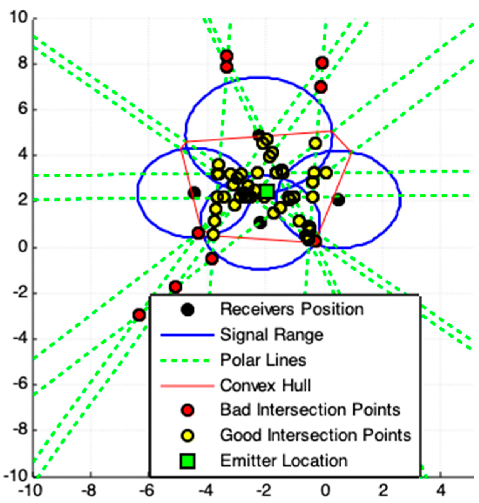
2.5. Tangent Lines Intersections Model (TLI)
| Algorithm 4. TLI—Tangent Lines Intersections Model Algorithm |
| Data Input |
| is the number of receivers. , , is the planar position of each receiver. , is the signal range of each receiver to an emitter. |
| Procedure |
| 1: for each |
| 2: , by (d-6) and (d-7), for each receiver position , used as pole-points, compute all combinations of polar-points and with the respective receiver at position and signal range . |
| 3: Stores the points and in the set . |
| 4: For each corresponding and polar-points, by (d-6), computes the respective two tangent lines equation and that passes by each . |
| 5: end for |
| 6: For all and tangent-lines, by (d-3), computes the intersections points, , among all tangent-lines. Store these intersections points in . |
| 7: Apply (d-8), find the convex hull polygon for all polar-points in . The obtained polygon is the minimal convex polygon that involves all interest points in . This polygon constitutes our ROI. |
| 8: Exclude from all intersections points among all tangent-lines on the boundary, or out, of the ROI, called bad intersections points. |
| 9: Apply (d-9), compute the location estimation, , of the emitter. |
| Information Output |
| 10: Emitter location estimation . |
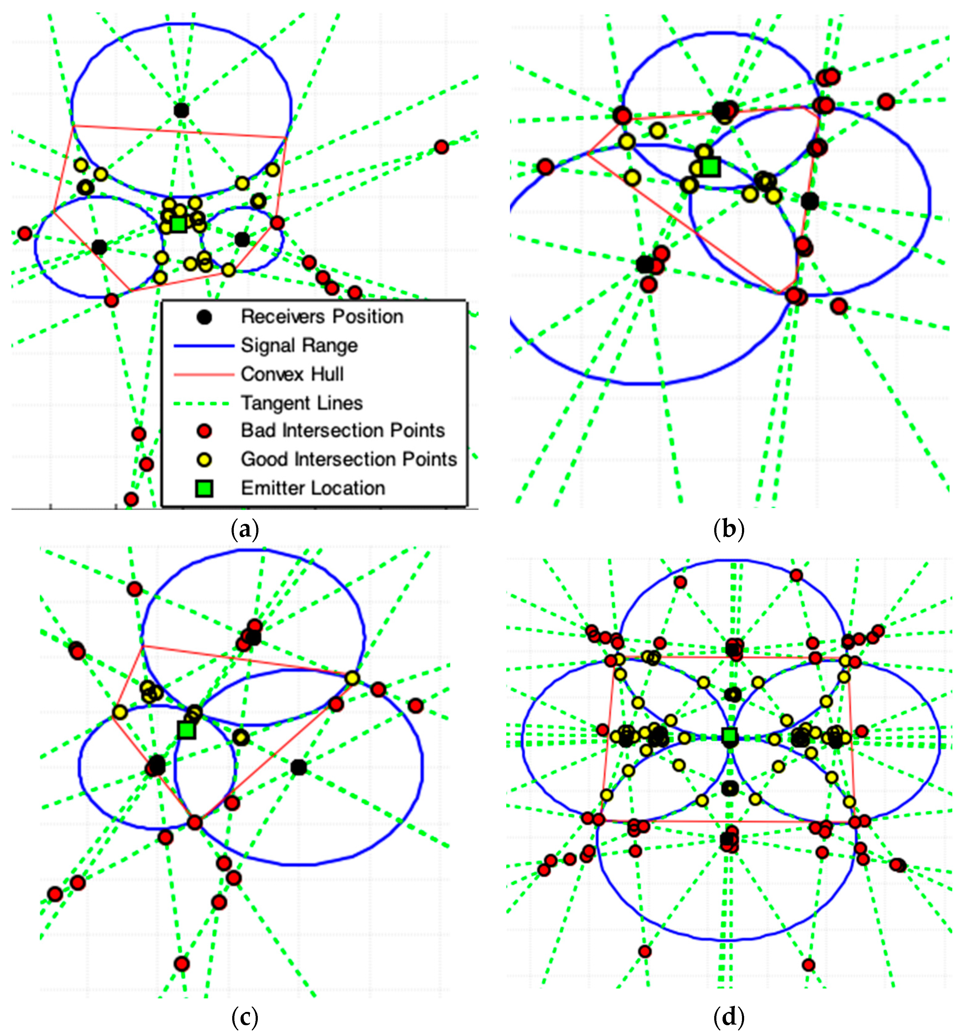
2.6. Tangent Lines with Minimal Angles Model (MAI)
| Algorithm 5. MAI—Tangent Lines with Minimal Angles Intersections Model Algorithm |
| Data Input |
| is the number of receivers. , , is the planar position of each receiver. , is the signal range of each receiver to an emitter. |
| Procedure |
| 1: for each |
| 2: , by (d-6) and (d-7), for each receiver position , used as pole-points, compute all combinations of polar-points and with the respective receiver at position and signal range . |
| 3: Stores the points and in the set . |
| 4: For each corresponding and polar-points, by (d-6), compute the respective two tangent lines equation and that passes by . |
| 5: end for |
| 6: For all and tangent-lines, by (d-3), compute the intersections points, , among all tangent-lines. Stores these intersections points in . |
| 7: Apply (d-8), find the convex hull polygon for all center circles points . The obtained polygon is the minimal convex polygon that involves all interest points in . This polygon constitutes our ROI. |
| 8: Exclude from all intersections points among all tangent-lines on the boundary, or out, of the ROI, called bad intersections points. |
| 9: Apply (d-9), compute the location estimation, , of the emitter. |
| Information Output |
| 10: Emitter location estimation . |
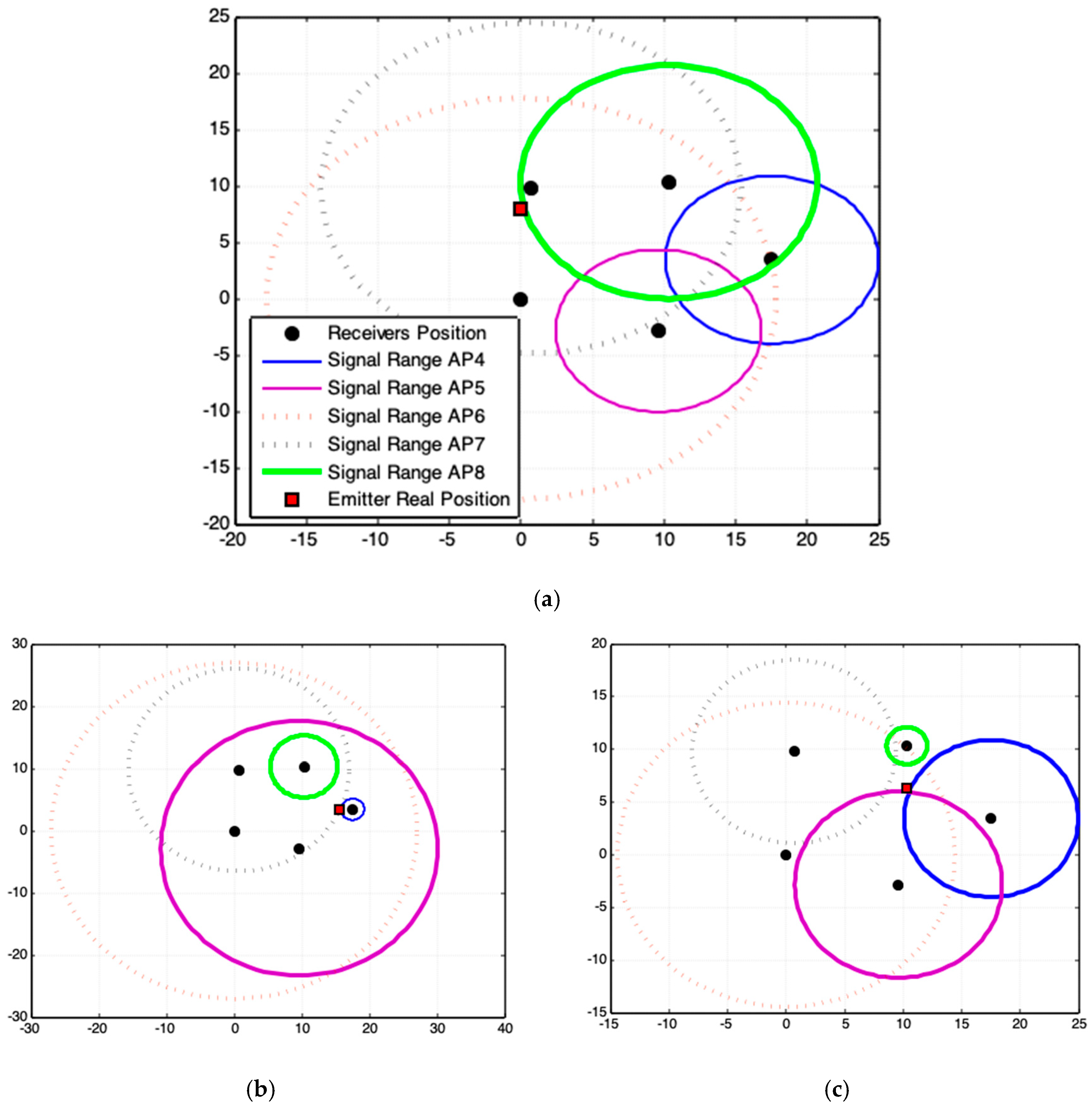
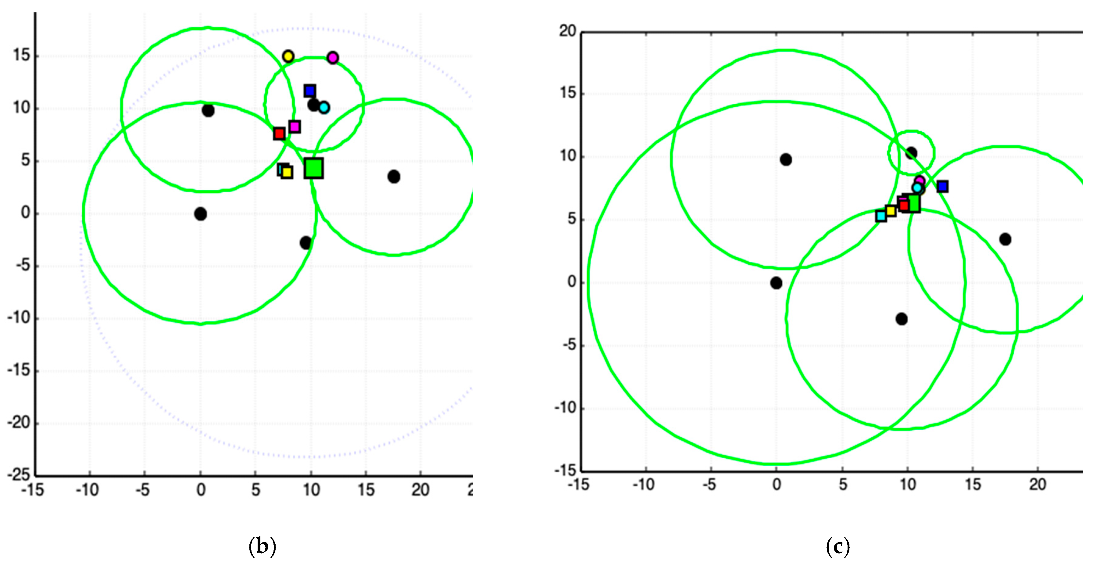
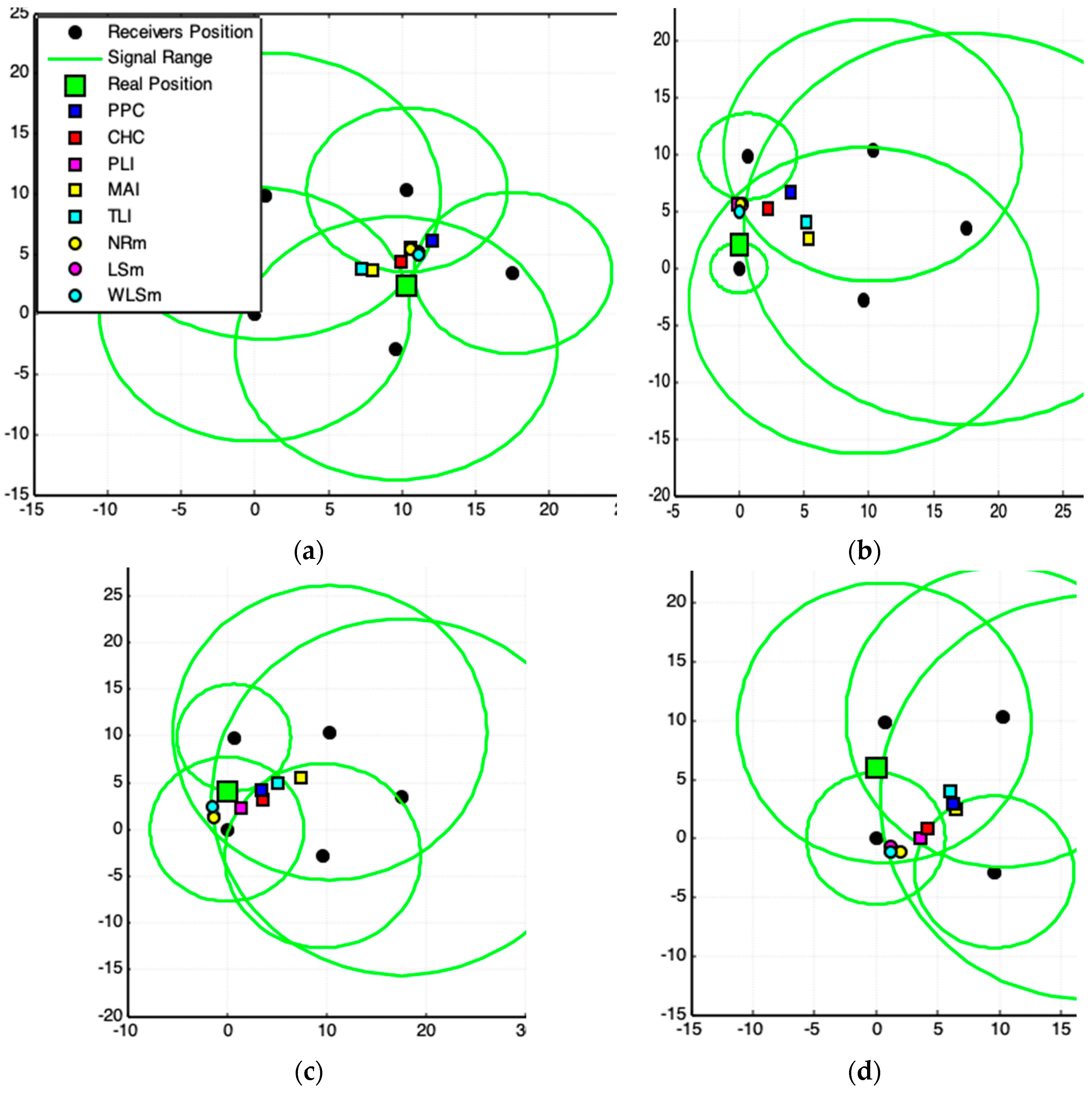
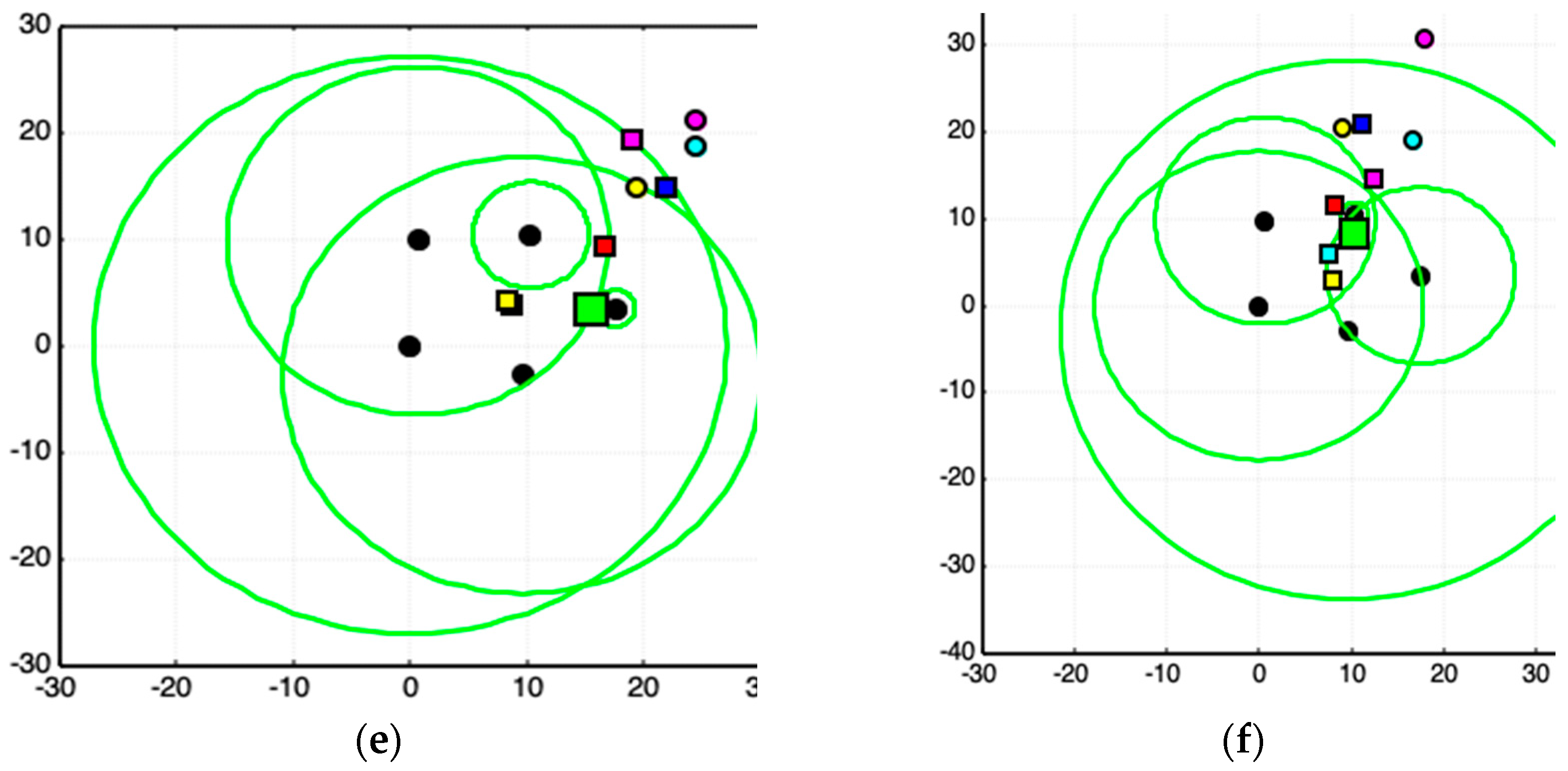
3. Experimental Cases
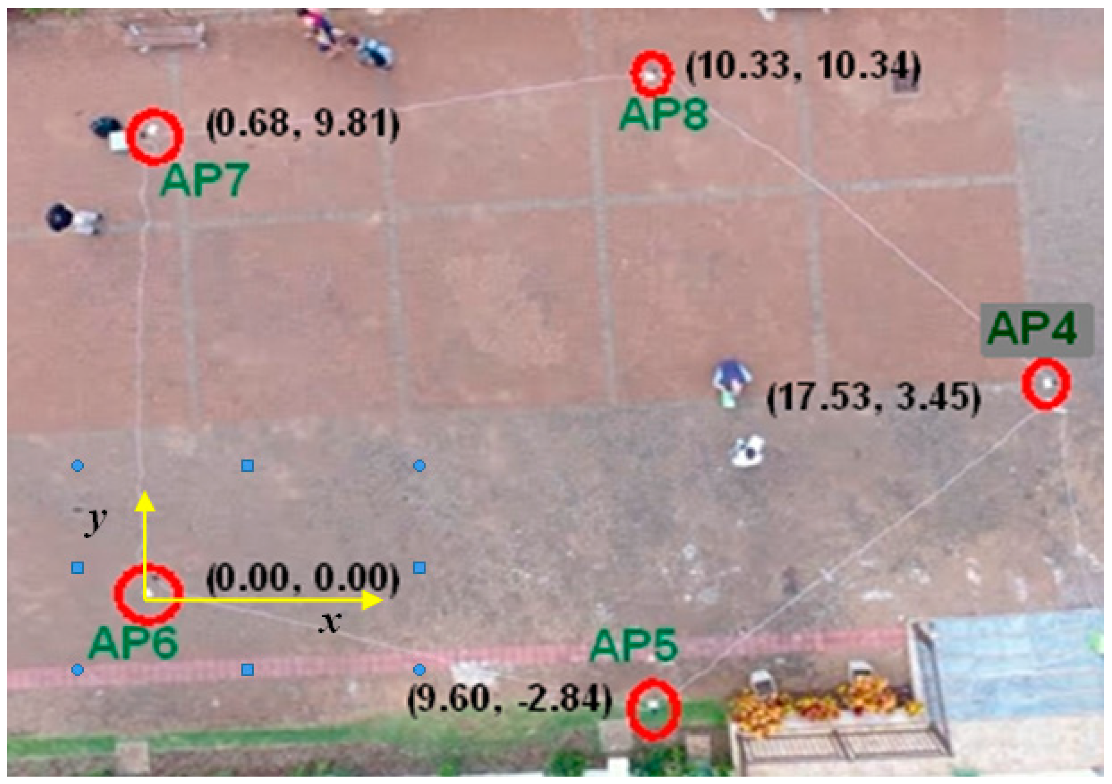
3.1. Methodology Applied to Real Data Acquisition
3.2. Quality of Acquired Data
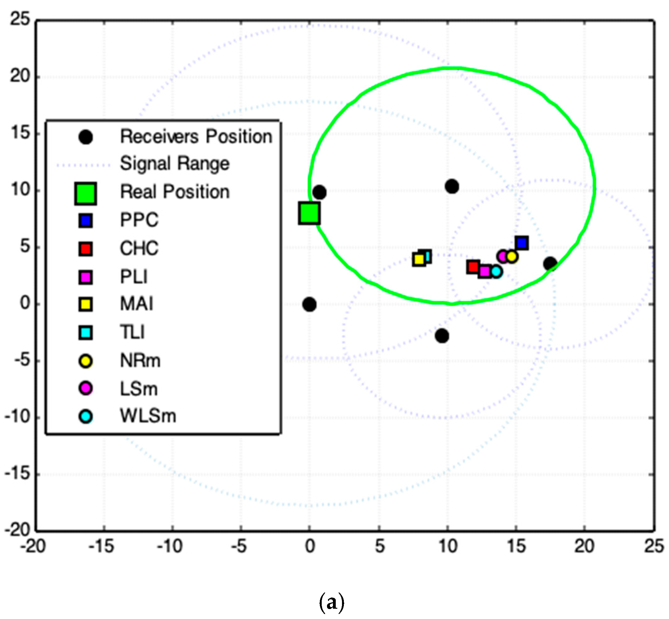
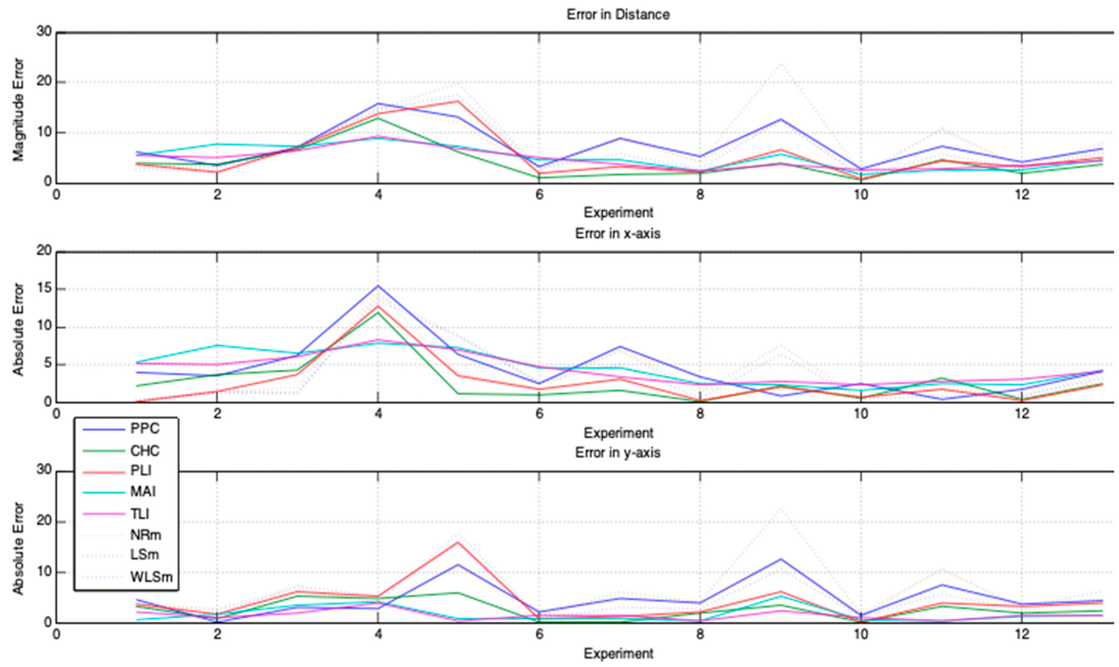
3.3. Results and Analyses
- PPC—Polar Points Centroid Model (proposed).
- CHC—Convex Hull Centroid Model (proposed).
- PLI—Polar Lines Intersections Model (proposed).
- TLI—Tangent Lines Intersections Model (proposed).
- MAI—Tangent Lines with Minimal Angles Model (proposed).
- NRm—Newton–Rapson Method (for comparison).
- LSm—Least Square Method (for comparison).
- WLSm—Weighted Least Square Method (for comparison).
4. Conclusions
Author Contributions
Funding
Acknowledgments
Conflicts of Interest
Appendix A. Complementary Results


References
- Wang, H.; Gao, Z.; Guo, Y.; Huang, Y. A Survey of Range-Based Localization Algorithms for Cognitive Radio Networks. In Proceedings of the Second International Conference on Consumer Electronics, Communications and Networks, Yichang, China, 21–23 April 2012; pp. 844–847. [Google Scholar] [CrossRef]
- O’Hara, B.; Petrick, A. The IEEE 802.11 Handbook: A Designers Companion, 2nd ed.; IEEE Press: New York, NY, USA, 2005; ISBN 0-7381-4449-5. [Google Scholar]
- Ahmad, U.; Gavrilov, A.V.; Lee, S.; Lee, Y.-K. A modular classification model for received signal strength based location systems. Neurocomput. Lett. 2008, 71, 2657–2669. [Google Scholar] [CrossRef]
- Kaemarungsi, K.; Krishnamurthy, P. Analysis of WLAN’s received signal strength indication for indoor location fingerprinting. Pervasive Mob. Comput. 2012, 8, 292–316. [Google Scholar] [CrossRef]
- Balanis, C.A.; Polycarpou, A.C. Antennas. Wiley Encyclopedia of Telecommunications; Proakis, J.G., Ed.; John Wiley & Sons: New York, NY, USA, 2003; pp. 179–188. [Google Scholar]
- Goswami, S. Indoor Location Technologies; Springer: Heidelberg, Germany, 2013; ISBN 978-1-4614-1377-6. [Google Scholar]
- Acharya, R. Understanding Satellite Navigation; Elsevier Inc.: Atlanta, GA, USA, 2014; Chapters 6–7; ISBN 978-0-12-799949-4. [Google Scholar] [CrossRef]
- Wu, R.H.; Lee, Y.H.; Tseng, H.W.; Jan, Y.G.; Chuang, M.H. Study of characteristics of RSSI signal. In Proceedings of the IEEE International Conference on Industrial Technology, ICIT 2008, Chengdu, China, 21–24 April 2008. [Google Scholar] [CrossRef]
- Fosdick, L.D.; Jessup, E.R.; Schauble, C.J.C.; Domik, G. An Introduction to High-Performance Scientific Computing; The MIT Press: Cambridge, MA, USA, 1996; ISBN 0-262-06181-3. [Google Scholar]
- Bahl, P.; Padmanabhan, V.N. RADAR: An in-building RF-based user location and tracking system. Proc. IEEE Infocom 2000, 2, 775–784. [Google Scholar]
- Maass, H. Location-Aware Mobile Applications based on Directory Services. In Proceedings of the 3rd Annual ACM/IEEE International Conference on Mobile Computing and Networking, MobiCom ’97, Budapest, Hungary, 26–30 September 1997; pp. 23–33, ISBN 0-89791-988-2. [Google Scholar] [CrossRef]
- Nelson, G.J. Context-Aware and Location Systems. Ph.D. Thesis, University of Cambridge, Computer Lab, Cambridge, UK, January 1998. [Google Scholar]
- CISCO. Wi-Fi Location-Based Services 4.1 Design Guide. 2014. Available online: http://www.cisco.com/c/en/us/td/docs/solutions/Enterprise/Mobility/WiFiLBS-DG.html (accessed on 13 February 2018).
- Mehra, R.; Singh, A. Real Time RSSI Error Reduction in Distance Estimation Using RLS Algorithm. In Proceedings of the IEEE 3rd International Advance Computing Conference, IACC 2013, Ghaziabad, India, 22–23 February 2013; pp. 661–665. [Google Scholar] [CrossRef]
- Luo, M.; Chen, X.; Cao, S.; Zhang, X. Two New Shrinking-Circle Methods for Source Localization Based on TDoA Measurements. Sensors 2018, 18, 1274. [Google Scholar] [CrossRef] [PubMed]
- Beutel, J. Location Management in Wireless Sensor Networks. In Handbook of Sensors Networks: Compact Wireless and Wired Sensing Systems; Ilyas, M., Mahgoub, I., Eds.; CRC Press: New York, NY, USA, 2005; ISBN 0-8493-1968-4. [Google Scholar]
- Tarrío, P.; Bernardos, A.M.; Casar, J.R. Weighted Least Squares Techniques for Improved Received Signal Strength Based Localization. Sensors 2011, 11, 8569–8592. [Google Scholar] [CrossRef] [PubMed]
- Atkinson, K.E. An Introduction to Numerical Analysis, 2nd ed.; John Wiley & Sons: New York, NY, USA, 1988; ISBN 978-0-471-62489-9. [Google Scholar]
- Bancroft, S. An algebraic solution of the GPS equations. IEEE Trans. Aerosp. Electron. Syst. 1985, AES-21, 56–59. [Google Scholar] [CrossRef]
- Strang, G.; Borre, K. Linear Algebra, Geodesy, and GPS; Wellesley Press: Cambridge, UK, 1997; ISBN 0961408863. [Google Scholar]
- Rahman, M.Z. Beyond Trilateration: GPS Positioning Geometry and Analytical Accuracy, Global Navigation Satellite Systems: Signal, Theory and Applications; Jin, S., Ed.; InTechOpen: London, UK, 2012; Chapter 10; pp. 241–256. ISBN 978-953-307-843-4. Available online: http://www.intechopen.com/books/global-navigation-satellite-systems-signal-theory-and-applications (accessed on 10 January 2018).
- WCIPEG—Programming Enrichment Group. Computational Geometry. Woburn Collegiate Institute’s. Available online: http://wcipeg.com/wiki/Computational_geometry (accessed on 13 February 2018).
- Gibson, C.G. Elementary Euclidean Geometry: An Introduction; Cambridge University Press: Cambridge, UK, 2004; ISBN 978-0-521-83448-3. [Google Scholar]
- Knuth, D.E. Axioms And Hulls: Lecture Notes in Computer Science; Springer: Heidelberg, Germany, 1992; ISBN 978-3-540-55611-4. [Google Scholar]
- Barber, C.B.; Dobkin, D.P.; Huhdanpaa, H.T. The Quickhull Algorithm for Convex Hulls. ACM Trans. Math. Softw. 1996, 22, 469–483. [Google Scholar] [CrossRef]
- O’Rourke, J. Computational Geometry in C, 2nd ed.; Cambridge University Press: Cambridge, UK, 1994; ISBN 978-0521649766. [Google Scholar]
- Halder, S.J.; Choi, T.Y.; Park, J.H.; Kang, S.H.; Park, S.W.; Park, J.G. Enhanced ranging using adaptive filter of ZIGBEE RSSI and LQI measurement. In Proceedings of the 10th International Conference on Information Integration and Web-Based Applications & Services, iiWAS ’08, Linz, Austria, 24–26 November 2008; pp. 367–373, ISBN 978-1-60558-349-5. [Google Scholar] [CrossRef]
- Elnahrawy, E.; Li, X.; Martin, R.P. The limits of localization using signal strength: A comparative study. In Proceedings of the Sensor and Ad Hoc Communications and Networks, Santa Clara, CA, USA, 4–7 October 2004; pp. 406–414. [Google Scholar]
- Wang, C.; Xiao, L. Sensor Localization under Limited Measurement Capabilities. IEEE Netw. 2007, 21, 16–23. [Google Scholar] [CrossRef]
- Mensing, C.; Plass, S. Positioning algorithms for cellular networks using TDOA. In Proceedings of the 2006 IEEE International Conference on Acoustics, Speech and Signal Processing, Toulouse, France, 14–19 May 2006; p. IV. [Google Scholar] [CrossRef]
- Wu, D.; Bao, L.; Li, R. UWB-Based Localization in Wireless Sensor Networks. Int. J. Commun. Netw. Syst. Sci. 2009, 2, 407–442. [Google Scholar] [CrossRef]
- Sahoo, P.K.; Hwang, I.-S. Collaborative Localization Algorithms for Wireless Sensor Networks with Reduced Localization Error. Sensors 2011, 11, 9989–10009. [Google Scholar] [CrossRef] [PubMed]
- Amitangshu, P. Localization Algorithms in Wireless Sensor Networks: Current Approaches and Future Challenges. Netw. Protoc. Algorithms 2010, 2, 45–73. [Google Scholar] [CrossRef]
- Schneider, C.; Zutz, S.; Rehrl, K.; Brunaue, R.; Gröchenig, S. Evaluating GPS sampling rates for pedestrian assistant. J. Locat. Based Serv. 2016, 10, 212–239. [Google Scholar] [CrossRef]
- Lam, L.D.M.; Tang, A.; Grundy, J. Heuristics-based indoor positioning systems: A systematic literature review. J. Locat. Based Serv. 2016, 10, 212–239. [Google Scholar] [CrossRef]
- Montanha, A.; Escalona, M.J.; Domínguez-Mayo, F.J.; Polidorio, A. Technological Innovation to Safely Aid in the Spatial Orientation of Blind People in a Complex Urban Environment. In Proceedings of the International Conference on Image, Vision and Computing (ICIVC), Portsmouth, UK, 3–5 August 2016; IEEE Publisher: New York, NY, USA, 2016; pp. 102–107. [Google Scholar] [CrossRef]


| Methods | Magnitudes Errors (in Meters) | ||||||||
|---|---|---|---|---|---|---|---|---|---|
| Minimum Error | Maximum Error | Mean Error | |||||||
| x-axis | y-axis | Distance | x-axis | y-axis | Distance | x-axis | y-axis | Distance | |
| PPC * | 0.4 | 0.2 | 2.7 | 15.5 | 12.5 | 15.7 | 4.2 | 4.4 | 6.9 |
| CHC * | 0.1 | 0.1 | 0.6 | 11.9 | 6.0 | 12.8 | 2.5 | 2.4 | 3.7 |
| PLI * | 0.1 | 0.1 | 0.7 | 12.8 | 15.9 | 16.3 | 2.4 | 3.8 | 5.0 |
| MAI * | 1.6 | 0.3 | 1.7 | 7.9 | 5.3 | 8.9 | 4.2 | 1.5 | 4.7 |
| TLI * | 2.3 | 0.3 | 2.3 | 8.3 | 3.9 | 9.2 | 4.1 | 1.3 | 4.4 |
| NRm | 0.1 | 1.1 | 1.3 | 14.7 | 12.2 | 15.2 | 2.8 | 5.1 | 6.5 |
| LSm | 0.3 | 1.2 | 1.8 | 14.1 | 22.5 | 23.7 | 3.6 | 6.4 | 7.9 |
| WLSm | 0.1 | 0.7 | 1.3 | 13.6 | 15.3 | 17.7 | 3.5 | 4.9 | 6.5 |
| Mean Errors (in Meters) | |||
|---|---|---|---|
| x-axis | y-axis | Distance | |
| Geometric Models | 3.7 | 2.9 | 5.3 |
| NRm + LSm+ WLSm | 3.5 | 4.1 | 6.0 |
| Methods | Standard Deviation of the Errors | Effective Variabilityof the Errors | ||
|---|---|---|---|---|
| x-axis | y-axis | Distance | ||
| PPC * | 4.1 | 3.8 | 4.5 | 4.1 |
| CHC * | 3.1 | 2.1 | 3.4 | 2.9 |
| PLI * | 3.3 | 4.1 | 4.9 | 4.1 |
| MAI * | 2.5 | 1.6 | 2.6 | 2.2 |
| TLI * | 2.3 | 1.0 | 2.3 | 1.9 |
| NRm | 4.0 | 4.0 | 4.9 | 4.3 |
| LSm | 4.3 | 6.7 | 7.4 | 6.1 |
| WLSm | 4.2 | 4.3 | 5.5 | 4.7 |
© 2019 by the authors. Licensee MDPI, Basel, Switzerland. This article is an open access article distributed under the terms and conditions of the Creative Commons Attribution (CC BY) license (http://creativecommons.org/licenses/by/4.0/).
Share and Cite
Montanha, A.; Polidorio, A.M.; Dominguez-Mayo, F.J.; Escalona, M.J. 2D Triangulation of Signals Source by Pole-Polar Geometric Models. Sensors 2019, 19, 1020. https://doi.org/10.3390/s19051020
Montanha A, Polidorio AM, Dominguez-Mayo FJ, Escalona MJ. 2D Triangulation of Signals Source by Pole-Polar Geometric Models. Sensors. 2019; 19(5):1020. https://doi.org/10.3390/s19051020
Chicago/Turabian StyleMontanha, Aleksandro, Airton M. Polidorio, F. J. Dominguez-Mayo, and María J. Escalona. 2019. "2D Triangulation of Signals Source by Pole-Polar Geometric Models" Sensors 19, no. 5: 1020. https://doi.org/10.3390/s19051020
APA StyleMontanha, A., Polidorio, A. M., Dominguez-Mayo, F. J., & Escalona, M. J. (2019). 2D Triangulation of Signals Source by Pole-Polar Geometric Models. Sensors, 19(5), 1020. https://doi.org/10.3390/s19051020