1. Introduction
Sight distances play an important role in road design. In fact, road design must help vehicles to stop safely, given breaking capacities, as soon as the driver sees a vehicle stopping in the same lane.
Passing maneuvers are another example of sight distance applications in road design. When passing is allowed, the road design must ensure that the driver can have enough space to complete a passing maneuver given the available sight distance.
These constrains are also applicable to autonomous or automated vehicles. In fact, given its sensing capabilities, the vehicle must run smoothly, perform overtaking safely or be able to stop if a car stops in its current lane. Sight distances have impact on vertical and horizontal alignments of road elements [
1]. It influences horizontal curve design, crest vertical curve design or road grades.
Sight distances are influenced by the height of scene perception sensors, i.e., a LiDAR (Light Detection And Ranging), a camera or the driver eye. Today’s standards use the average height of driver eyes. For instance, the 2011 edition of AASHTO (American Association of State Highway and Transportation Officials) Greenbook uses height of the driver’s eye equal to 1.08 m (3.54 ft) [
2] based on Fambro study [
3]. It was 1.65 m (5.41 ft), 1.15 m (3.77 ft), 1.07 m (3.51 ft) in 1920, 1965 and 2000 editions, respectively. The height of the driver eye used in the UK is 1.05 m (3.45 ft) and relies on [
4].
The height of the target also has an impact on sight distances. Headlights or taillights are often considered as targets for sight distance computations. The 2011 AASHTO Geometric design guide [
2] suggests an object height of 600 mm (2.0 ft) for stopping and decision sight distances and 1080 mm (3.55 ft) for passing and intersection sight distances The height of object height in the UK ranges from 0.25 m (0.82 ft) to 2.0 m (6.56 ft).
For the time being, French regulations use a height of a driver’s eye of 1 m (3.28 ft) and the height of target objects of 0.6 m (1.97 ft) [
5]). They were set in 2000. Both heights were defined based on car manufacturer data sheets and a survey carried out at a toll station close to Paris. The height of target objects of 0.6 m was consistent between both sources of information. The height of target objects corresponds to the 10th percentile of the height distribution of the rear tail light lower limit of the emitting area. The survey carried out at the toll station did not allow to accurately measure the height of the driver’s eye. As a result, the Fambro study [
3] was used to define the height of driver’s eye. The height of 1 m was chosen as it represents the 2.5th percentile.
Few studies have investigated how to obtain and update the height of driver eyes standards. Approaches can be empirical. In [
3], Fambro et al. used a color camera. They placed markers on the road to be used as a scale and drove vehicles with known heights for calibration purposes. In 2012, Reference [
6] proposed to use the car model to find out the height of driver eyes. The camera is placed in a parallel fashion with the side plane of the vehicle. The vehicle height is used to scale the driver’s eye height measurement. Methods can also be analytical. In [
7], the researchers used a two-step approach. First, the Society of Automotive Engineering (SAE) standard on seating reference point (SgRP) is used. Then, the UMTRI (University of Michigan Transportation Research Institute) eyellipse model, based on the observations of 68 drivers collected in a lab environment, is used in conjunction with the SgRP to obtain eye height distribution.
Our work addresses the problem of empirical height measurements from camera-based temporary roadside measurements. We aim at proposing a framework that is versatile enough to measure the height from one camera but could also provide other information such as the lateral location of the vehicle on the road if necessary. It must be robust and requires high repeatability. The process is automatic except for the selection of the point required to find the object of interest’s height. It will have to locate 3D points in the scene.
Measuring the height from the location of 3D points in the scene requires to obtain the extrinsic calibration, i.e., the location of the camera with respect to the ground plane and the traffic direction. As mentioned in [
8], calibration patterns do not naturally exist in traffic scenes. Consequently, there is a growing interest in automatic calibration from CCTV cameras. Reference [
9] relies on vanishing points to find out the camera orientation with respect to the ground plane. The traffic’s main direction and gradients from the vehicles are used to find the vanishing points.
Zheng and Peng go a step further as they estimate both intrinsic and extrinsic parameters [
8]. They also relied on vanishing points to estimate the camera orientation. Several approaches are proposed to recover the camera translation with respect to the road plane origin. Overall, CCTVs are placed far from the ground [
10]. Consequently, the camera field of view covers a large area. The car trajectory can be observed for a long period. Moreover, the three main directions from cuboid-like car shape can easily be seen.
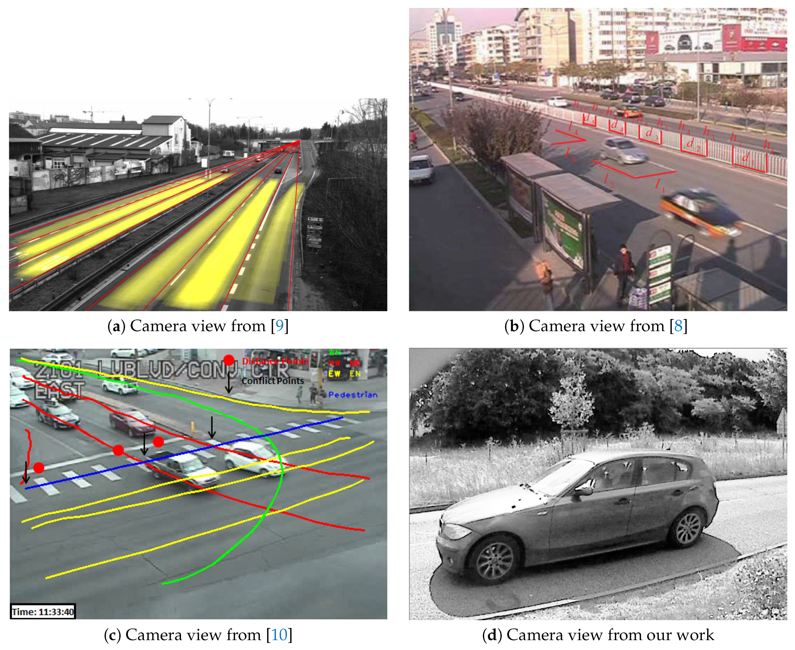
As it can be seen in
Figure 1d and Figure 4b, measurements from ground level and temporary setups are not so convenient. In fact, high posts may not frequently exist in the environment. Moreover, regulation requires using guy-wire for temporary high posts. A larger space is required for guy-wire that might not be available at the measurement location.
Consequently, our work proposes a framework that allows to measure heights in traffic scenes from ground level cameras. Our method does not require the traffic to be stopped. Our approach is suitable for temporary setups in any road environments (urban, road side, ...) and works both in daytime or low illumination situations.
The paper is organized as follows.
Section 2 presents a flexible framework that allows to locate 3D points on the car.
Section 3 first qualifies the performance of our approach on the vehicle height task and presents the height of driver eyes and taillight distribution.
Section 4 concludes the paper.
2. Methodology
A camera is a sensor that images the world with the help of a lens and an image sensor. The image is a perspective projection of the world. The camera model relates a 3D point and its 2D projection as follows:
where:
is a 3D point in the World frame.
is the projection of P in the image.
is a scaling factor.
is the transformation that brings point from the world coordinate system to the camera coordinate system. R and t are also known as extrinsic parameters.
K is the transformation that brings point from the camera coordinate system to the image frame.
K embeds the intrinsic parameters of the camera:
where:
s and
r are considered respectively equal to 0 and 1 [
11].
Equation (
1) is applicable to perfect cameras. For real cameras, the lens quality and misalignment between the lens and the image sensor may introduce deformations in the resulting image called distortions. Consequently, Equation (
1) must be modified as follows:
where:
The intrinsic parameters as well as the distortion coefficients can be recovered with a camera calibration. Standard camera calibration approaches include works from [
12] and [
13].
Measuring the height from an image from 3D information requires to measure the distance from the ground to the point of interest. Consequently, the intrinsic and extrinsic parameters must be known as well as the scaling factor. Unfortunately, the scaling factor is lost due to the projective property of the transformation.
The best that can be recovered from a pixel in an image is a 3D line that passes through the origin of the camera coordinate system and the back projection of the pixel on the unit plane.
In the example given in
Figure 2c,
p cannot be recovered. However, only the line (black line) passes through
p and the camera’s coordinate system origin can be recovered as follows:
Still, we do not know how far the 3D point is on the line from a single image, Consequently, in order to recover object heights from a single image, either several cameras must be used or a single camera with a-priori information. As it can be seen in
Figure 2, the road can be approximated as a plane defined by the normal
. A vehicle can be represented by a cuboid. We consider that the vehicle vertical axis is parallel to the road plane normal. In order to measure the height, we must find the location of the car frame origin with respect to the camera frame. The car can be anywhere on the road platform. However, car motions are mainly in the same directions, i.e., the longitudinal direction.
In order to obtain a method that does not require knowing the car model, we applied a three-step approach. The key information are the directions of , and in the camera frame as well as the location of the ground plane. One could try to detect the vehicle edges in order to find these parameters. However, with today’s car designs, it would be highly inaccurate to try to estimate the direction from the roof or the door edges. Moreover, the location of the car frame origin is still missing.
In order to obtain robust and accurate estimations of , and , we employ a checkerboard.
The checkerboard is placed vertically on the road platform as shown in
Figure 2a. As it can be seen
,
and
are respectively parallel to
,
and
. The checkerboard origin is located at the top-left corner of the checkerboard.
First, we must find the location of the checkerboard frame in the camera frame. In other words, the transformation that relates the camera frame and the checkerboard frame must be found. Checkerboards are classic patterns used in camera calibration processes. Standard calibration techniques estimate the intrinsic parameters from several views of a checkerboard patterns as well as the extrinsic calibration, i.e., the location and orientation of each checkerboards in the camera frame.
In order to obtain good results, it is better to have a checkerboard that covers a large part of the image. Moreover, it is highly advised to have different orientations of the checkerboard to achieve robust intrinsic parameter estimation. In our case, the calibration is performed under traffic. As a result, only small time-windows are available to place the checkerboard. We favored one good pose of the checkerboard that we record over a small amount of time (up to 5 s). This single pose will result in a poor calibration. It will be even worst because the checkerboard size in the image would be rather small.
All things considered, we first calibrate the camera in a lab. Consequently, the intrinsic parameters are accurately estimated with a retro-projection error of less than one pixel despite lens distortions. Still, we must estimate the pose of the checkerboard in 3D from its projection in the image, i.e., 2D points.
This problem is known as the perspective-n-point proble m (PnP problem). PnP solving require at least three-point correspondences. It is a well-established problem. Several approaches can be found in literature from the computer vision community [
14,
15,
16,
17]. Consequently, the rotation matrix R and translation vector t from the camera frame to the checkerboard frame are obtained by solving the PnP problem. The pipeline summary is presented in
Figure 3.
It allows to find the directions
as follows:
As the checkerboard frame origin is not located at the ground level, the coordinate of the ground point is given as:
where:
3D planes are geometrical object algebraically defined by a 1 × 4 vector P =
. A 3D point X =
belonging to the plane must fulfill:
where:
Thanks to our PnP solution, the ground plane normal is already known. In fact, as it can be seen in
Figure 2,
and
are parallel. As a result,
is equal to
.
d can be easily obtained as it must solve:
We are consequently able to recover the ground plane definition in the camera frame with:
We have gathered all the information required to start the measurements. As it can be seen in
Figure 2c,
is parallel to
and
to
.
Figure 2c explains how we recover the 3D height from 2D image points. First, a pixel as close as possible to the contact of the vehicle wheel with the ground, represented as
, must be chosen. It defines
, the normalize point coordinate of the selected pixel. A second pixel corresponding to the object projection from which we want to know the height, represented as
, must be chosen resulting in
once in normalized coordinates.
and
actually represents two 3D directions represented as orange and purple lines respectively. We first use
to find the location of the vehicle side plane. We have to find the intersection of the purple line with the ground plane found previously.
is computed as follows:
allows to find the lateral position of the vehicle side plane
. As done previously with
, we use the normal directions found with the checkerboard. The vehicle side plane definition is given by:
We are consequently able to recover the side plane
definition in the camera frame with:
Finally, we use
to recover
as follows:
may not be vertically aligned with
. As a result, we considered the height of
as the distance of
to the ground plane
:


