A Novel Deep Learning Method for Intelligent Fault Diagnosis of Rotating Machinery Based on Improved CNN-SVM and Multichannel Data Fusion

 , ,
, ,
Abstract
:1. Introduction
2. Standard Convolutional Neural Network
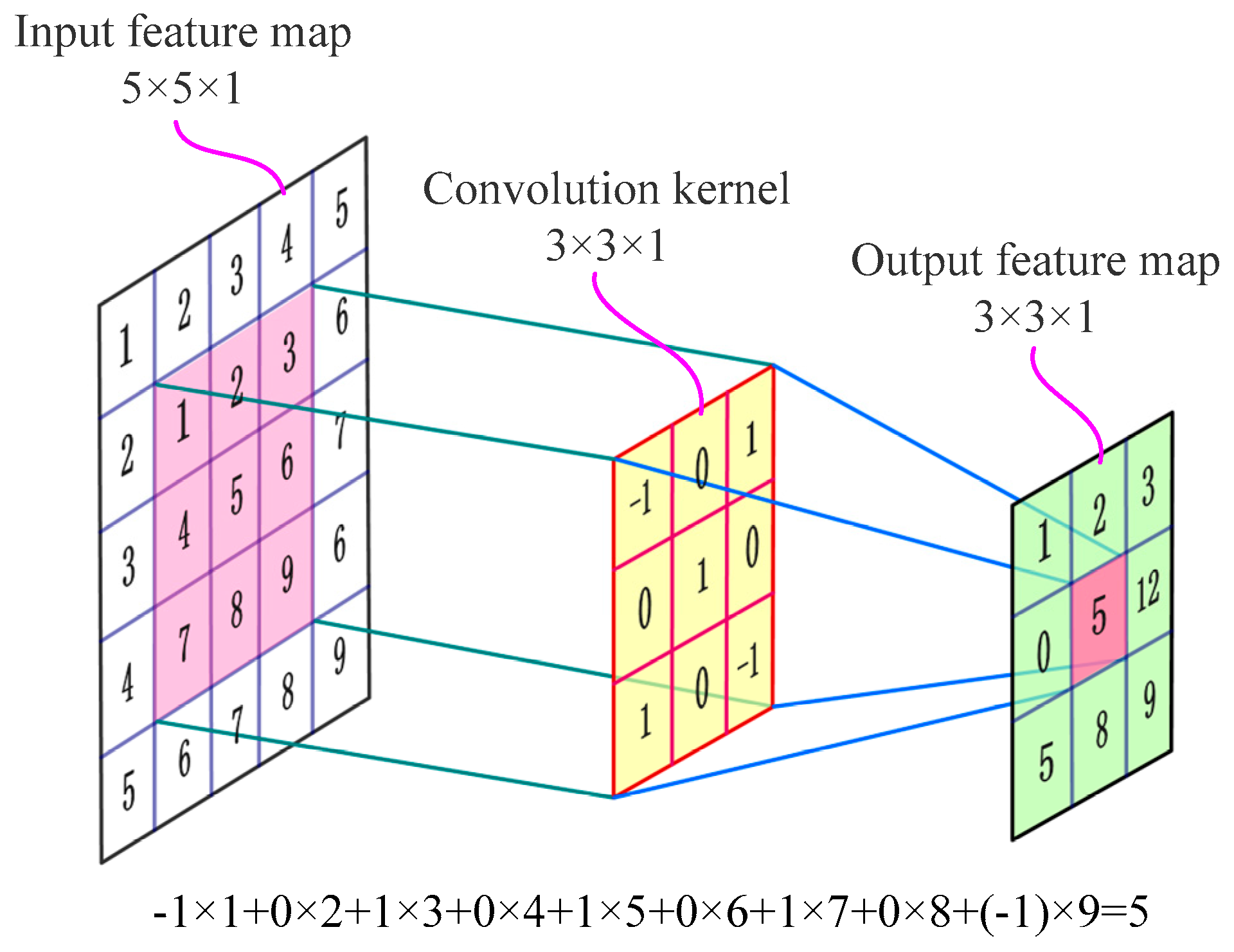
2.1. Convolution Operation Layer
2.2. Activation Operation Layer
2.3. Pooling Operation Layer
2.4. Fully Connection Layer
3. The Improved CNN-SVM Intelligent Fault Diagnosis Method
3.1. Improved CNN-SVM Algorithm Construction
3.2. Intelligent Fault Diagnosis Based on Improved CNN-SVM Method
3.3. Deep Learning Training Skills
4. Experimental Verification Based on Multichannel Vibration Signals
4.1. Multichannel Fusion Fault Dataset of Rolling Bearing
4.2. Fault Data Processing
4.3. Hyper-Parameters Selection of CNN Model
4.4. Fault Diagnosis Results and Evaluate of Proposed CNN-SVM Model
4.5. Comparison with Other Intelligent Algorithms
5. Conclusions
Author Contributions
Funding
Conflicts of Interest
References
- Liu, R.; Yang, B.; Zio, E.; Chen, X. Artificial intelligence for fault diagnosis of rotating machinery: A review. Mech. Syst. Signal Process. 2018, 108, 33–47. [Google Scholar] [CrossRef]
- Zhang, W.; Li, C.; Peng, G.; Chen, Y.; Zhang, Z. A deep convolutional neural network with new training methods for bearing fault diagnosis under noisy environment and different working load. Mech. Syst. Signal Process. 2018, 100, 439–453. [Google Scholar] [CrossRef]
- Shao, H.; Jiang, H.; Ying, L.; Li, X. A novel method for intelligent fault diagnosis of rolling bearings using ensemble deep auto-encoders. Mech. Syst. Signal Process. 2018, 102, 278–297. [Google Scholar] [CrossRef]
- Xia, M.; Li, T.; Xu, L.; Liu, L.; de Silva, C.W. Fault diagnosis for rotating machinery using multiple sensors and convolutional neural networks. IEEE/ASME Trans. Mech. 2018, 23, 101–110. [Google Scholar] [CrossRef]
- Lei, Y.; Jia, F.; Zhou, X.; Lin, J. A deep learning-based method for machinery health monitoring with big data. J. Mech. Eng. 2015, 51, 49–56. [Google Scholar] [CrossRef]
- Wen, C.; Lv, F.; Bao, Z.; Liu, M. A review of data driven-based incipient fault diagnosis. Acta Autom. Sin. 2016, 42, 1285–1299. [Google Scholar]
- Amar, M.; Gondal, I.; Wilson, C. Vibration spectrum imaging: A novel bearing fault classification approach. IEEE Trans. Ind. Electron. 2015, 62, 494–502. [Google Scholar] [CrossRef]
- Harmouche, J.; Delpha, C.; Diallo, D. Incipient fault detection and diagnosis based on Kullback-Leibler divergence using principal component analysis: Part II. Signal Process. 2015, 109, 334–344. [Google Scholar] [CrossRef]
- Yu, G.; Xing, W.; Jing, N.; Rong, F.F. Incipient faults identification in gearbox by combining kurtogram and independent component analysis. Appl. Mech. Mater. 2015, 764, 309–313. [Google Scholar]
- Nguyen, V.H.; Seshadrinath, J.; Wang, D.; Nadarajan, S.; Vaiyapuri, V. Model-based diagnosis and rul estimation of induction machines under inter-turn fault. IEEE Trans. Ind. Appl. 2017, 53, 2690–2701. [Google Scholar] [CrossRef]
- Wen, L.; Li, X.; Gao, L.; Zhang, Y. A new convolutional neural network-based data-driven fault diagnosis method. IEEE Trans. Ind. Electron. 2018, 65, 5990–5998. [Google Scholar] [CrossRef]
- Du, X.; Li, Z.; Chen, G.; Hu, J.; Hu, D. Application analysis on vibration monitoring system of three gorges hydropower plant. J. Hydroelectr. Eng. 2016, 35, 77–92. [Google Scholar]
- Rubini, R.; Meneghetti, U. Application of the envelope and wavelet transform analyses for the diagnosis of incipient faults in ball bearings. Mech. Syst. Signal Process. 2001, 15, 287–302. [Google Scholar] [CrossRef]
- Muruganatham, B.; Sanjith, M.A.; Krishnakumar, B.; Murty, S.A.V.S. Roller element bearing fault diagnosis using singular spectrum analysis. Mech. Syst. Signal Process. 2013, 35, 150–166. [Google Scholar] [CrossRef]
- Huang, N.E. New method for nonlinear and nonstationary time series analysis: Empirical mode decomposition and Hilbert spectral analysis. Proc. SPIE 2000, 4056, 197–209. [Google Scholar]
- Li, H.; Zhang, Q.; Qin, X.; Sun, Y. Fault diagnosis method for rolling bearings based on short-time Fourier transform and convolution neural network. J. Vib. Shock 2018, 37, 124–131. [Google Scholar]
- Yu, Y.; Yu, D.; Cheng, J. A roller bearing fault diagnosis method based on EMD energy entropy and ANN. J. Sound Vib. 2006, 294, 269–277. [Google Scholar] [CrossRef]
- Jegadeeshwaran, R.; Sugumaran, V. Fault diagnosis of automobile hydraulic brake system using statistical features and support vector machines. Mech. Syst. Signal Process. 2015, 52, 436–446. [Google Scholar] [CrossRef]
- Yao, D.; Yang, J.; Cheng, X.; Wang, X. Railway rolling bearing fault diagnosis based on muti-scale IMF permutation entropy and SA-SVM Classifier. J. Mech. Eng. 2018, 54, 168–176. [Google Scholar] [CrossRef]
- Islam, M.; Lee, G.; Hettiwatte, S. Incipient fault diagnosis in power transformers by clustering and adapted KNN. In Proceedings of the 2016 Australasian Universities Power Engineering Conference, Brisbane, Australia, 25–28 September 2016; pp. 1–5. [Google Scholar]
- Qu, J.; Yu, L.; Yuan, T.; Tian, Y.; Gao, F. Adaptive fault diagnosis algorithm for rolling bearings based on one-dimensional convolutional neural network. Chin. J. Sci. Instrum. 2018, 39, 134–143. [Google Scholar]
- Hinton, G.; Salakhutdinov, R. Reducing the dimensionality of data with neural networks. Science 2006, 313, 504–507. [Google Scholar] [CrossRef]
- Goodfellow, I.; Bengio, Y.; Courville, A. Deep Learning; MIT Press: Cambridge, MA, USA, 2016. [Google Scholar]
- Schmidhuber, J. Deep learning in neural networks: An overview. Neural Netw. 2015, 61, 85–117. [Google Scholar] [CrossRef]
- Noda, K.; Yamaguchi, Y.; Nakadai, K.; Okuno, H.G.; Ogata, T. Audio-visual speech recognition using deep learning. Appl. Intell. 2015, 42, 722–737. [Google Scholar] [CrossRef]
- Zhang, Y.; Dong, Z.; Chen, X.; Jia, W.; Du, S.; Muhammad, K.; Wang, S. Image based fruit category classification by 13-layer deep convolutional neural network and data augmentation. Multimedia Tools Appl. 2019, 78, 3613–3632. [Google Scholar] [CrossRef]
- Young, T.; Hazarika, D.; Poria, S.; Cambria, E. Recent trends in deep learning based natural language processing. IEEE Comput. Intell. Mag. 2018, 13, 55–75. [Google Scholar] [CrossRef]
- Jiao, F.; Lei, Y.; Lin, J. Deep neural networks: A promising tool for fault characteristic mining and intelligent diagnosis of rotating machinery with massive data. Mech. Syst. Signal Process. 2016, 72, 303–315. [Google Scholar] [CrossRef]
- Tamilselvan, P.; Wang, P. Failure diagnosis using deep belief learning based health state classification. Reliab. Eng. Syst. Saf. 2013, 115, 124–135. [Google Scholar] [CrossRef]
- Li, W.; Shan, W.; Zeng, X. Bearing fault identification based on deep belief network. J. Vib. Eng. 2016, 29, 340–347. [Google Scholar]
- Lecun, Y.; Bottou, L.; Bengio, Y.; Haffner, P. Gradient-based learning applied to document recognition. Proc. IEEE 1998, 86, 2278–2324. [Google Scholar] [CrossRef]
- David, V.; Ferrada, A.; Droguett, E.; Viviana, M.; Mohammad, M. Deep learning enabled fault diagnosis using time-frequency image analysis of rolling element bearings. Shock Vib. 2017, 2017, 1–17. [Google Scholar]
- Zhang, W.; Peng, G.; Li, C. Bearings fault diagnosis based on convolutional neural networks with 2-D representation of vibration signals as input. In Proceedings of the 2016 the 3rd International Conference on Mechatronics and Mechanical Engineering (ICMME 2016), Shanghai, China, 21–23 October 2016; pp. 1–5. [Google Scholar]
- Lin, M.; Chen, Q.; Yan, S. Network in network. In Proceedings of the International Conference on Learning Representations, Banff, AB, Canada, 14–16 April 2014; pp. 1–10. [Google Scholar]
- Lecun, Y.; Bengio, Y.; Hinton, G. Deep learning. Nature 2015, 521, 436–444. [Google Scholar] [CrossRef]
- Deng, L.; Yu, D. Deep learning: methods and applications. Found. Trends Signal Process. 2014, 7, 197–387. [Google Scholar] [CrossRef]
- LeCun, Y.; Kavukcuoglu, K.; Farabet, C. Convolutional networks and applications in vision. In Proceedings of the 2010 IEEE International Symposium on Circuits and Systems, Paris, France, 30 May–2 June 2010; pp. 253–256. [Google Scholar]
- Su, Q.; Liao, X.; Carin, L. A probabilistic framework for nonlinearities in stochastic neural networks. In Proceedings of the 31st Conference on Neural Information Processing Systems, Long Island, NY, USA, 4–9 December 2017; pp. 1–10. [Google Scholar]
- Wang, L.; Xie, Y.; Zhou, Z. Asynchronous motor fault diagnosis based on convolutional neural network. J. Vib. Meas. Diagn. 2017, 6, 1208–1215. [Google Scholar]
- Simonyan, K.; Zisserman, A. Very deep convolutional networks for large-scale image recognition. arXiv, 2014; arXiv:1409.1556. [Google Scholar]
- Jiang, M.; Liang, Y.; Feng, X.; Fan, X.; Pei, Z.; Xue, Y.; Guan, R. Text classification based on deep belief network and softmax regression. Neural Comput. Appl. 2018, 29, 61–70. [Google Scholar] [CrossRef]
- Flach, P. Machine Learning; Cambridge University Press: Cambridge, UK, 2012. [Google Scholar]
- Szegedy, C.; Liu, W.; Jia, Y.; Sermanet, P.; Reed, S.; Anguelov, D.; Erhan, D.; Vanhoucke, V.; Rabinovich, A. Going deeper with convolutions. In Proceedings of the 2015 IEEE Conference on Computer Vision and Pattern Recognition (CVPR), Boston, MA, USA, 7–12 June 2015; pp. 1–9. [Google Scholar]
- Hoang, D.; Kang, H. Rolling element bearing fault diagnosis using convolutional neural network and vibration image. Cognit. Syst. Res. 2019, 53, 42–50. [Google Scholar] [CrossRef]
- Chen, Q. Research Related to Support Vector Machines. Ph.D. Thesis, Ocean University of China, Shandong province, China, 2011. [Google Scholar]
- Wang, S.; Muhammad, K.; Hong, J.; Sangaiah, A.; Zhang, Y. Alcoholism identification via convolutional neural network based on parametric ReLU, dropout, and batch normalization. Neural Comput. Appl. 2018, 6, 1–16. [Google Scholar] [CrossRef]
- Montserrat, D.M.; Qian, L.; Allebach, J.; Delp, E. Training object detection and recognition CNN models using data augmentation. Electron. Imaging 2017, 2017, 27–36. [Google Scholar] [CrossRef]
- Srivastava, N.; Hinton, G.; Krizhevsky, A.; Sutskever, I.; Salakhutdinov, R. Dropout: A simple way to prevent neural networks from overfitting. J. Mach. Learn. Res. 2014, 15, 1929–1958. [Google Scholar]
- Kingma, D.; Ba, J. Adam: A method for stochastic optimization. arXiv, 2014; arXiv:1412.6980. [Google Scholar]
- Gong, W.; Huang, M.; Zhang, M.; Mo, Q. Multi-objective optimization of bonding head based on sensitivity and analytic hierarchy process. J. Vib. Shock 2015, 34, 128–134. [Google Scholar]
- Bearing Data Center. Available online: http://csegroups.case.edu/bearingdatacenter/home (accessed on 20 October 2018).
- Guo, X.; Chen, L.; Shen, C. Hierarchical adaptive deep convolution neural network and its application to bearing fault diagnosis. Measurement 2016, 93, 490–502. [Google Scholar] [CrossRef]


| Function Name | Sigmoid | Tanh | Relu |
|---|---|---|---|
| expressions | |||
| graphs |  |  |  |
| Parameter Type | Inside Diameter | Outside Diameter | Thickness | Ball Diameter | Pitch Diameter |
|---|---|---|---|---|---|
| Size: (inches) | |||||
| Drive end bearing | 0.9843 | 2.0472 | 0.5906 | 0.3126 | 1.5370 |
| Fan end bearing | 0.6693 | 1.5748 | 0.4724 | 0.2656 | 1.1220 |
| Class Label | Fault Location | Fault Size (inches) | Fault Severity | Sample Length | Sample Number |
|---|---|---|---|---|---|
| 0 | Normal | None | None | 500 × 2 | 200 × 3 |
| 1 | Ball | Diameter: 0.007, Depth: 0.011 | incipient fault (F−) | 500 × 2 | 200 × 3 |
| 2 | Ball | Diameter: 0.014, Depth: 0.011 | moderate fault (F) | 500 × 2 | 200 × 3 |
| 3 | Ball | Diameter: 0.021, Depth: 0.011 | significant fault (F+) | 500 × 2 | 200 × 3 |
| 4 | Inner Raceway | Diameter: 0.007, Depth: 0.011 | incipient fault (F−) | 500 × 2 | 200 × 3 |
| 5 | Inner Raceway | Diameter: 0.014, Depth: 0.011 | moderate fault (F) | 500 × 2 | 200 × 3 |
| 6 | Inner Raceway | Diameter: 0.021, Depth: 0.011 | significant fault (F+) | 500 × 2 | 200 × 3 |
| 7 | Outer Raceway | Diameter: 0.007, Depth: 0.011 | incipient fault (F−) | 500 × 2 | 200 × 3 |
| 8 | Outer Raceway | Diameter: 0.014, Depth: 0.011 | moderate fault (F) | 500 × 2 | 200 × 3 |
| 9 | Outer Raceway | Diameter: 0.021, Depth: 0.011 | significant fault (F+) | 500 × 2 | 200 × 3 |
| Class Label | Fault Location | Sample Length | Sample Number | Training Dataset | Verification Dataset | Testing Dataset |
|---|---|---|---|---|---|---|
| 0 | Normal | 500 × 2 | 200 × 3 | 112 × 3 | 28 × 3 | 60 × 3 |
| 1 | Ball | 500 × 2 | 200 × 3 | 112 × 3 | 28 × 3 | 60 × 3 |
| 2 | Ball | 500 × 2 | 200 × 3 | 112 × 3 | 28 × 3 | 60 × 3 |
| 3 | Ball | 500 × 2 | 200 × 3 | 112 × 3 | 28 × 3 | 60 × 3 |
| 4 | Inner Raceway | 500 × 2 | 200 × 3 | 112 × 3 | 28 × 3 | 60 × 3 |
| 5 | Inner Raceway | 500 × 2 | 200 × 3 | 112 × 3 | 28 × 3 | 60 × 3 |
| 6 | Inner Raceway | 500 × 2 | 200 × 3 | 112 × 3 | 28 × 3 | 60 × 3 |
| 7 | Outer Raceway | 500 × 2 | 200 × 3 | 112 × 3 | 28 × 3 | 60 × 3 |
| 8 | Outer Raceway | 500 × 2 | 200 × 3 | 112 × 3 | 28 × 3 | 60 × 3 |
| 9 | Outer Raceway | 500 × 2 | 200 × 3 | 112 × 3 | 28 × 3 | 60 × 3 |
| Layer Type | Hyper-Parameter Settings | Output Shape | Learnable Parameters |
|---|---|---|---|
| Input layer | (batch, 25 × 20, 2) | (batch, 25 × 20, 2) | 0 |
| Convolution layer 1 | Filter = (3 × 3, 2, 64), strides = (1, 1), padding = “Same” | (batch, 25 × 20, 64) | 1216 |
| Activation layer 1 | activation function | (batch, 25 × 20, 64) | 0 |
| Max-Pooling layer 1 | Ksize = (1, 2 × 2, 1), strides = (2, 2), padding = “Same” | (batch, 12 × 10, 64) | 0 |
| Convolution layer 2 | Filter = (3 × 3, 64, 32), strides = (1, 1), padding = “Same” | (batch, 12 × 10, 32) | 18,464 |
| Activation layer 2 | activation function | (batch, 12 × 10, 32) | 0 |
| Max-Pooling layer 2 | Ksize = (1, 2 × 2, 1), strides = (2, 2), padding = “Same” | (batch, 6 × 5, 32) | 0 |
| Flatten layer | flatten Max-Pooling layer 2 to 1-D shape | (batch, 960) | 0 |
| FC-Dense layer 1 | 128 hidden layer neuron nodes | (batch, 128) | 123,008 |
| FC-Activation layer 1 | activation function | (batch, 128) | 0 |
| FC-Dense layer 2 | 10 hidden layer neuron nodes | (batch, 10) | 1290 |
| Softmax output layer | Softmax activation function | (batch, 10) | 0 |
| Serial Number | Convolution Layer 1 | Convolution Layer 2 | Fully Connected Layer | Accuracy | Training Time (s) | Test Time (s) |
|---|---|---|---|---|---|---|
| 1 | relu | relu | relu | 0.9768 | 117.104 | 0.1275 |
| 2 | tanh | tanh | tanh | 0.9814 | 120.652 | 0.1404 |
| 3 | sigmoid | sigmoid | sigmoid | 0.7309 | 121.302 | 0.1875 |
| 4 | relu | relu | tanh | 0.9897 | 117.392 | 0.1404 |
| 5 | relu | relu | sigmoid | 0.9692 | 124.728 | 0.1455 |
| 6 | sigmoid | sigmoid | relu | 0.3938 | 122.864 | 0.1572 |
| 7 | sigmoid | sigmoid | tanh | 0.3106 | 123.896 | 0.1704 |
| 8 | tanh | tanh | relu | 0.9683 | 123.924 | 0.1946 |
| 9 | tanh | tanh | sigmoid | 0.9692 | 123.416 | 0.1404 |
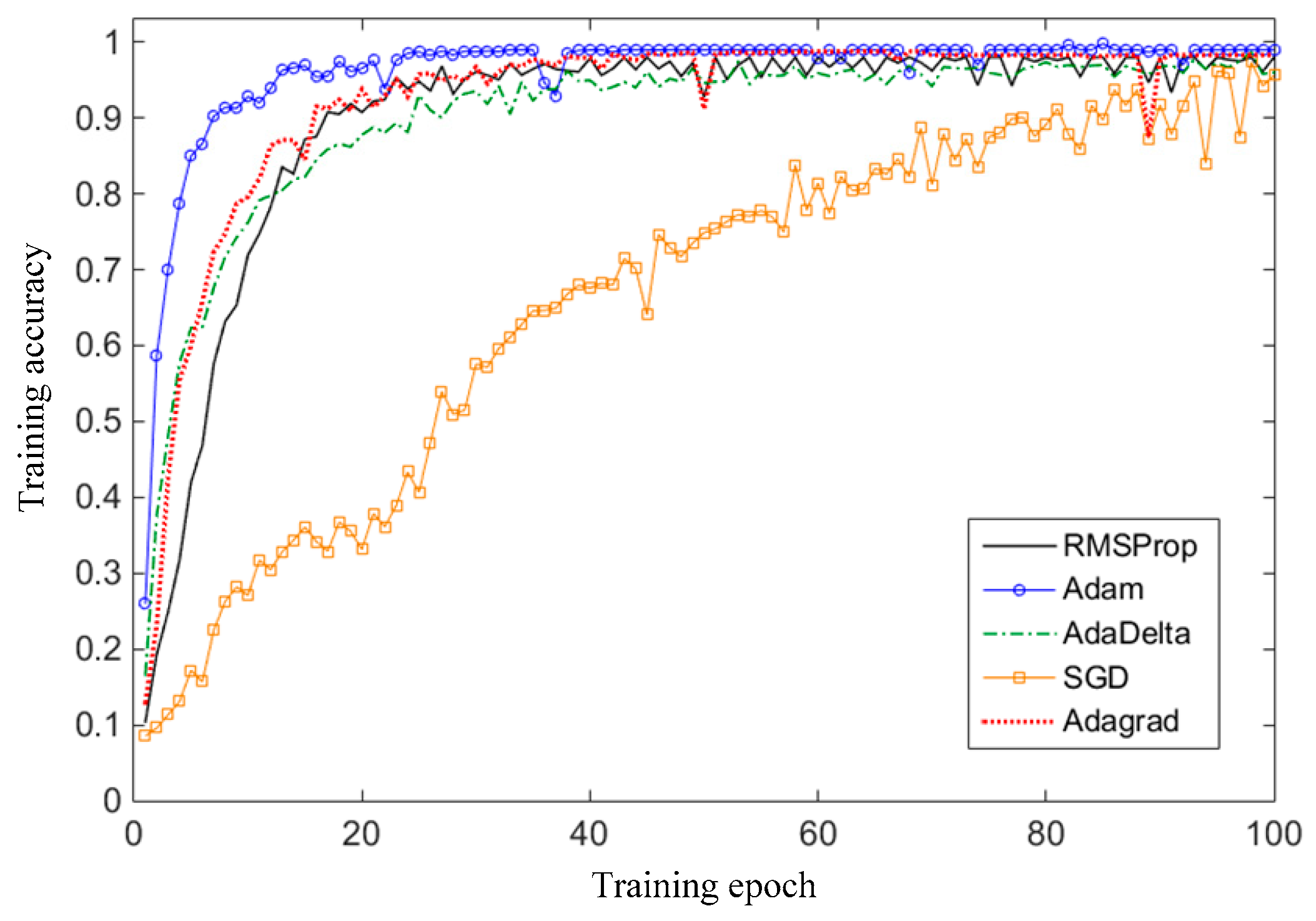
| Optimization Algorithm | Number of Iterations | Accuracy | Training Time (s) | Test Time (s) |
|---|---|---|---|---|
| SGD | 100 | 0.9276 | 123.172 | 0.18936 |
| Adagrad | 100 | 0.9882 | 117.912 | 0.17145 |
| AdaDelta | 100 | 0.9871 | 124.252 | 0.18351 |
| RMSProp | 100 | 0.9872 | 114.092 | 0.16842 |
| Adam | 100 | 0.9899 | 114.876 | 0.16739 |
| Mini-Batch Number | Accuracy | Average Training Time (s) |
|---|---|---|
| 1 | 0.9585 | 4286.88 |
| 8 | 0.9799 | 601.056 |
| 16 | 0.9872 | 324.976 |
| 32 | 0.9883 | 185.288 |
| 64 | 0.9899 | 114.876 |
| 128 | 0.9828 | 87.6292 |
| 256 | 0.9640 | 69.3592 |
| 512 | 0.8729 | 57.9404 |
| CNN | CNN Model Hyper-Parameters |
|---|---|
| L = 1 | Conv2d (3 × 3, 64) + Pooling (2 × 2) + Full Connect (128/10) + Softmax |
| Conv2d (3 × 3, 64) + Pooling (2 × 2) + Dropout (0.5) + Full Connect (128/10) + Softmax | |
| L = 2 | Conv2d (3 × 3, 64) + Pooling (2 × 2) + Conv2d (3 × 3, 32) + Pooling (2 × 2) + Full Connect (128/10) + Softmax |
| Data augmentation + Conv2d (3 × 3, 64) + Pooling (2 × 2) + Dropout (0.3) + Conv2d (3 × 3, 32) + Pooling (2 × 2) + Dropout (0.2) + Full Connect (128/10) + Softmax | |
| L = 3 | Data augmentation + Conv2d (3 × 3, 64) + Pooling (2 × 2) + Conv2d (3 × 3, 32) + Pooling (2 × 2) + Conv2d (3 × 3, 32) + Pooling (2 × 2) + Full Connect (128/10) + Softmax |
| Data augmentation + Conv2d (3 × 3, 64) + Pooling (2 × 2) + Dropout (0.3) + Conv2d (3 × 3, 32) + Pooling (2 × 2) + Dropout (0.2) + Conv2d (3 × 3, 32) + Pooling (2 × 2) + Dropout (0.2) + Full Connect (128/10) + Softmax |
| Model Structure | L1 | L2 | L3 |
|---|---|---|---|
| Test Accuracy | |||
| No training skills | 96.04% | 98.31% | 98.76% |
| Data augmentation + Dropout | 97.92% | 98.99% | 98.93% |
| CNN-Softmax Training Stage Model Structure | |||
|---|---|---|---|
| Layer Type | Parameter Settings | Output Shape | Learnable Parameters |
| Input layer | (batch, 25 × 20, 2) | (batch, 25 × 20, 2) | 0 |
| Convolution layer 1 | Filter = (3 × 3, 2, 64), strides = (1, 1), padding = “Same” | (batch, 25 × 20, 64) | 1216 |
| Activation layer 1 | ReLU activation function | (batch, 25 × 20, 64) | 0 |
| Max-Pooling layer 1 | ksize = (1, 2 × 2, 1), strides = (2, 2), padding = “Same” | (batch, 12 × 10, 64) | 0 |
| Dropout layer 1 | Dropout (0.3) | (batch, 12 × 10, 64) | 0 |
| Convolution layer 2 | filter = (3 × 3, 64, 32), strides = (1, 1), padding = “Same” | (batch, 12 × 10, 32) | 18,464 |
| Activation layer 2 | ReLU activation function | (batch, 12 × 10, 32) | 0 |
| Max-Pooling layer 2 | ksize = (1, 2 × 2, 1), strides = (2, 2), padding = “Same” | (batch, 6 × 5, 32) | 0 |
| Dropout layer 2 | Dropout (0.2) | (batch, 6 × 5, 32) | 0 |
| Convolution layer 3 | filter = (1 × 1, 32, 10), strides = (1, 1), padding = “Same” | (batch, 6 × 5, 10) | 330 |
| Global average pooling layer | ksize = (1, 5 × 4, 1), strides = (5, 4), padding = “Same” | (batch, 10) | 0 |
| CNN feature output layer | Save CNN model parameters | (batch, 10) | 0 |
| Softmax output layer | Softmax activation function | (batch, 10) | 0 |
| CNN-SVM test stage model structure | |||
| Input layer | (batch, 25 × 20, 2) | (batch, 25 × 20, 2) | 0 |
| CNN feature output layer | raw data input into trained CNN extraction features | (batch, 10) | 0 |
| SVM classification layer | Nonlinear SVM classifier | (batch, 10) | 110 |
| Final output layer | Fault diagnosis result | (batch, 10) | 0 |
| Layer Type | Traditional Fully Connected CNN Model | Improved CNN-SVM |
|---|---|---|
| Convolution layer 1 | 1216 | 1216 |
| Convolution layer 2 | 18,464 | 18,464 |
| Convolution layer 3 | None | 330 |
| FC-Dense layer 1 | 123,008 | None |
| FC-Dense layer 2 | 1290 | None |
| SVM classification layer | None | 110 |
| Total parameter amount | 143,978 | 20,120 |
| Model Name | Test Accuracy | Training Time (s) | Testing Time (s) |
|---|---|---|---|
| Improved CNN+Softmax | 99.12% | 73.8293 | 0.08967 |
| Improved CNN+SVM | 99.94% | 74.3205 | 0.08318 |
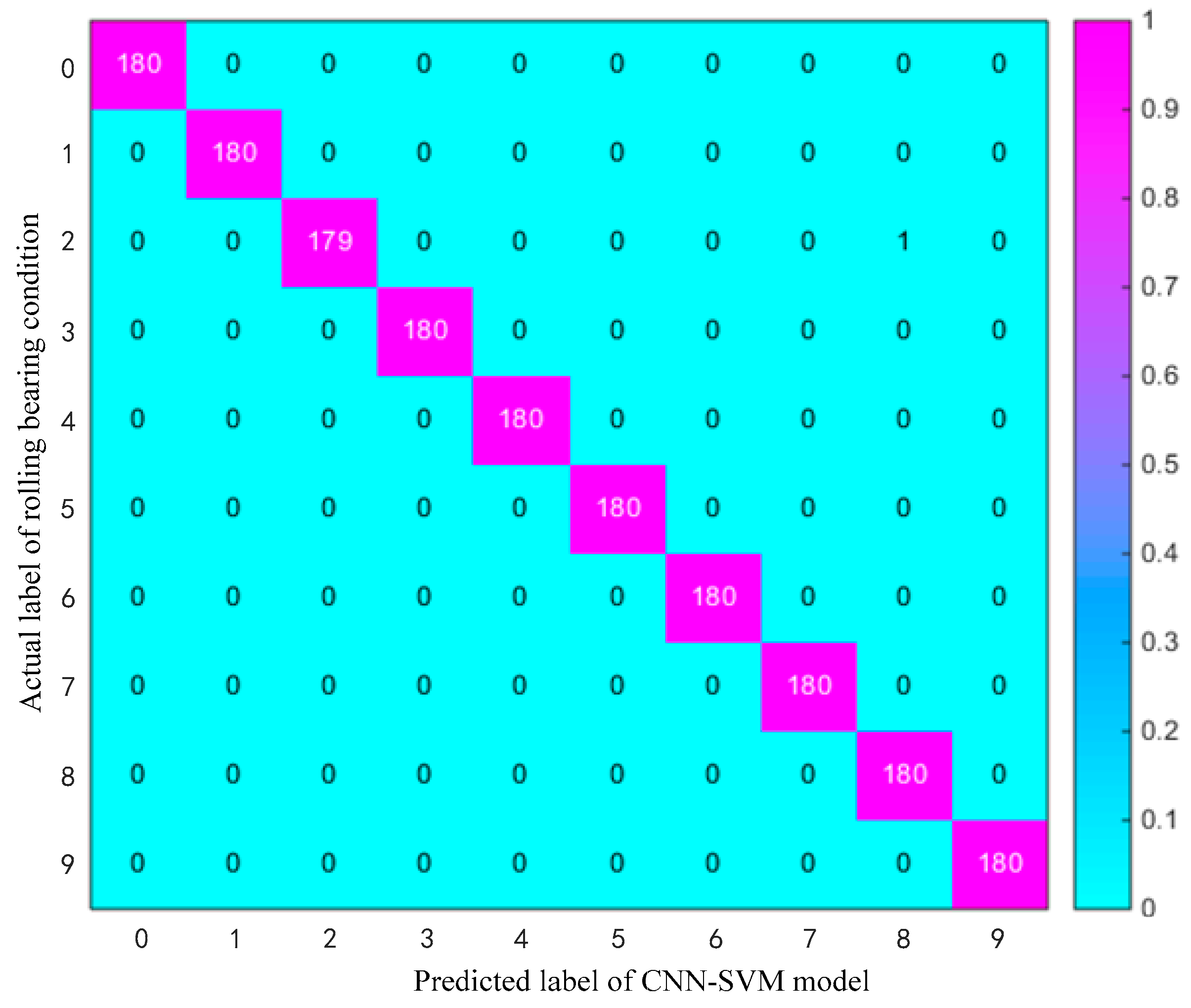
| Health Condition | Precision Rate | Recall Rate | F1-Measure | Sample Amount |
|---|---|---|---|---|
| Condition 0 | 100% | 100% | 100% | 180 |
| Condition 1 | 100% | 100% | 100% | 180 |
| Condition 2 | 100% | 99.44% | 99.72% | 180 |
| Condition 3 | 100% | 100% | 100% | 180 |
| Condition 4 | 100% | 100% | 100% | 180 |
| Condition 5 | 100% | 100% | 100% | 180 |
| Condition 6 | 100% | 100% | 100% | 180 |
| Condition 7 | 100% | 100% | 100% | 180 |
| Condition 8 | 99.45% | 100% | 99.72% | 180 |
| Condition 9 | 100% | 100% | 100% | 180 |
| Average/total | 99.94% | 99.94% | 99.94% | 1800 |
| Domain | Feature Parameters | |
|---|---|---|
| Time-domain | Absolute mean: | Crest factor: |
| Variance: | Root mean square: | |
| Crest: | Pulse factor: | |
| Clearance factor: | Skewness: | |
| Kurtosis: | Shape factor: | |
| Frequency-domain | Crest: | Mean energy: |
| Kurtosis: | Variance: | |
| Methods | ||||||||||||
|---|---|---|---|---|---|---|---|---|---|---|---|---|
| Bearing Condition | CNN-SVM | SVM | KNN | BPNN | DNN | CNN | ||||||
| P (%) | R (%) | P (%) | R (%) | P (%) | R (%) | P (%) | R (%) | P (%) | R (%) | P (%) | R (%) | |
| Condition 0 | 100 | 100 | 100 | 100 | 100 | 97.78 | 91.24 | 98.33 | 99.45 | 100 | 100 | 100 |
| Condition 1 | 100 | 100 | 89.67 | 91.67 | 98.29 | 95.56 | 90.66 | 91.67 | 76.50 | 99.44 | 95.72 | 99.44 |
| Condition 2 | 100 | 99.44 | 90.34 | 88.33 | 87.28 | 83.89 | 72.40 | 77.22 | 69.77 | 100 | 94.74 | 100 |
| Condition 3 | 100 | 100 | 86.75 | 80.01 | 91.47 | 65.56 | 75.01 | 45.01 | 93.33 | 54.44 | 100 | 90.56 |
| Condition 4 | 100 | 100 | 95.24 | 100 | 82.24 | 69.44 | 99.42 | 95.56 | 100 | 98.89 | 100 | 100 |
| Condition 5 | 100 | 100 | 98.85 | 95.56 | 84.11 | 100 | 100 | 100 | 100 | 89.44 | 100 | 100 |
| Condition 6 | 100 | 100 | 94.15 | 98.33 | 71.43 | 100 | 91.84 | 100 | 98.08 | 85.00 | 100 | 100 |
| Condition 7 | 100 | 100 | 99.45 | 100 | 100 | 100 | 64.98 | 92.78 | 100 | 93.89 | 100 | 100 |
| Condition 8 | 99.45 | 100 | 95.58 | 96.11 | 100 | 92.22 | 76.00 | 84.44 | 99.45 | 100 | 99.44 | 99.44 |
| Condition 9 | 100 | 100 | 99.45 | 100 | 96.72 | 98.33 | 77.97 | 51.11 | 100 | 98.33 | 100 | 100 |
| Average value | 99.94 | 99.94 | 94.95 | 95.01 | 91.15 | 90.28 | 83.95 | 83.61 | 93.66 | 91.94 | 98.99 | 98.94 |
© 2019 by the authors. Licensee MDPI, Basel, Switzerland. This article is an open access article distributed under the terms and conditions of the Creative Commons Attribution (CC BY) license (http://creativecommons.org/licenses/by/4.0/).
Share and Cite
Gong, W.; Chen, H.; Zhang, Z.; Zhang, M.; Wang, R.; Guan, C.; Wang, Q. A Novel Deep Learning Method for Intelligent Fault Diagnosis of Rotating Machinery Based on Improved CNN-SVM and Multichannel Data Fusion. Sensors 2019, 19, 1693. https://doi.org/10.3390/s19071693
Gong W, Chen H, Zhang Z, Zhang M, Wang R, Guan C, Wang Q. A Novel Deep Learning Method for Intelligent Fault Diagnosis of Rotating Machinery Based on Improved CNN-SVM and Multichannel Data Fusion. Sensors. 2019; 19(7):1693. https://doi.org/10.3390/s19071693
Chicago/Turabian StyleGong, Wenfeng, Hui Chen, Zehui Zhang, Meiling Zhang, Ruihan Wang, Cong Guan, and Qin Wang. 2019. "A Novel Deep Learning Method for Intelligent Fault Diagnosis of Rotating Machinery Based on Improved CNN-SVM and Multichannel Data Fusion" Sensors 19, no. 7: 1693. https://doi.org/10.3390/s19071693