Overcoming Bandwidth Limitations in Wireless Sensor Networks by Exploitation of Cyclic Signal Patterns: An Event-triggered Learning Approach


Abstract
:1. Introduction
- (i)
- The number of transmitted values (bits) per sampling instant can be reduced.
- (ii)
- The number of sampling instants with communication can be reduced.
- We extend ETL to multidimensional nonlinear system with cyclic excitation and a non-Euclidean state space. The states of the system are unit quaternions that represent body segment orientations.
- We propose an ETL algorithm that uses Gaussian process regression (GPR) for prediction and thereby reduces the communication load that is associated with model updates.
- We validate the proposed methods using real measurement data and compare the performance to those of more conventional or fundamentally different approaches, such as compression by adaptive differential pulse code modulation.
- We apply the method to data from a sensor network and investigate the effect of network delays and a limitation of the number of transmission channels.
1.1. Related Work
2. Specific Problem Setting
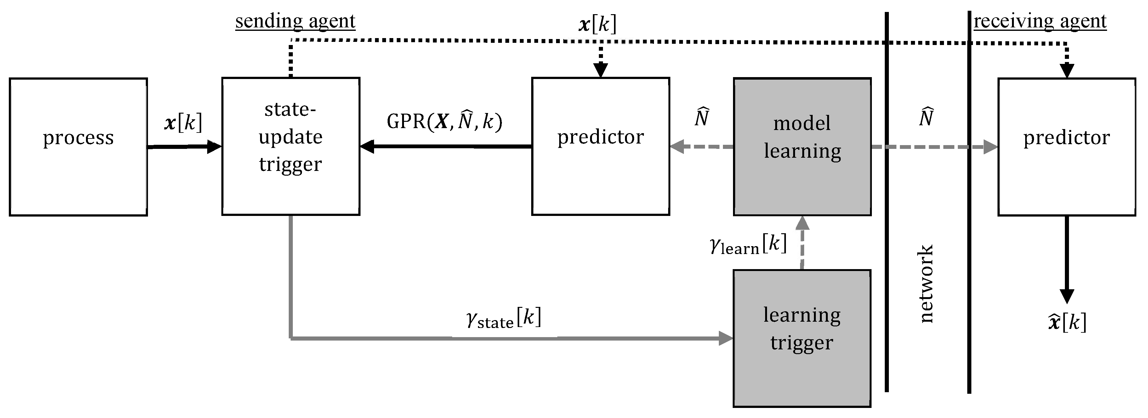
2.1. Setup
2.2. Goals
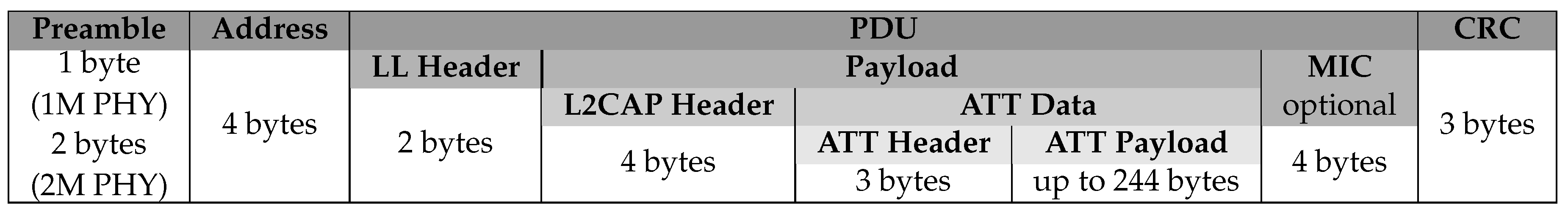
- The number of transmitted data bits, i.e., the size of the ATT Payload (cf. Figure 3).
- The number of sampling instants with data transmission, where is the indicator function.
- The total number of transmitted bits including the Bluetooth 5 overhead.
- The maximum absolute angle difference between the measured and the estimated body segment orientation , i.e., the upper error bound.
- The RMS-value of the error.
3. Methods
3.1. Orientation Representation
3.2. Event-Triggered Learning (ETL)
3.3. Hierarchical ETL
- Full model updates are updates of the whole trajectory .
- Small model updates adjust only a small number of parameters ; in the examined problem setting, the current trajectory is warped to the new cycle length and shifted by to obtain the new .
3.4. ETL with Gaussian Process Regression (GPR)
4. Experiments
- The first set (variable) contains approximately 4 min (180 steps) of simulated pathological gait with frequent style, speed, and ground inclination changes.
- The second set (steady) contains approximately 4 min (200 steps) of normal walking, at first with a speed of 2 km/h, then with 4 km/h.
4.1. Parameterization
4.2. Parameter Study
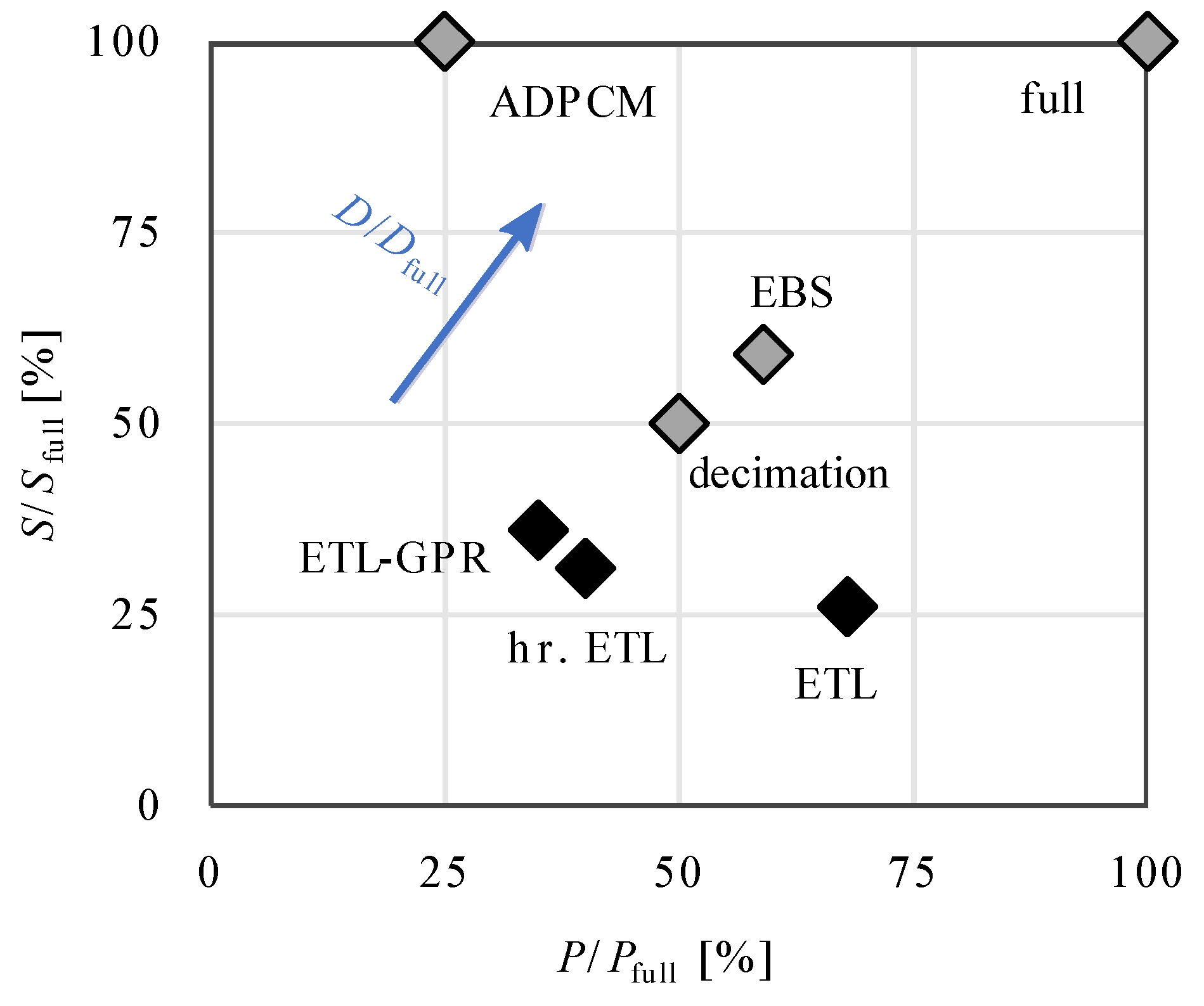
4.3. Performance Comparison
4.4. Different Body Segments
4.5. Delayed Model Identification and Transmission
4.6. Limited Number of Channels
5. Discussion
5.1. Method Comparison
5.2. Sensor Networks
5.3. Limitations
5.4. Comparison with Related Work
6. Conclusions
Author Contributions
Funding
Conflicts of Interest
References
- Giggins, O.M.; Persson, U.M.; Caulfield, B. Biofeedback in rehabilitation. J. Neuroeng. Rehabil. 2013, 10, 60. [Google Scholar] [CrossRef] [PubMed] [Green Version]
- Schwartz, M. (Ed.) Biofeedback; IntechOpen: London, UK, 2018. [Google Scholar]
- Huen, D.; Liu, J.; Lo, B. An integrated wearable robot for tremor suppression with context aware sensing. In Proceedings of the IEEE 13th International Conference on Wearable and Implantable Body Sensor Networks (BSN), San Francisco, CA, USA, 14–17 June 2016; pp. 312–317. [Google Scholar]
- Schicketmueller, A.; Rose, G.; Hofmann, M. Feasibility of a Sensor-Based Gait Event Detection Algorithm for Triggering Functional Electrical Stimulation during Robot-Assisted Gait Training. Sensors 2019, 19, 4804. [Google Scholar] [CrossRef] [PubMed] [Green Version]
- Seel, T.; Werner, C.; Schauer, T. The adaptive drop foot stimulator–Multivariable learning control of foot pitch and roll motion in paretic gait. Med Eng. Phys. 2016, 38, 1205–1213. [Google Scholar] [CrossRef] [PubMed]
- Teufl, W.; Lorenz, M.; Miezal, M.; Taetz, B.; Fröhlich, M.; Bleser, G. Towards inertial sensor based mobile gait analysis: Event-detection and spatio-temporal parameters. Sensors 2019, 19, 38. [Google Scholar] [CrossRef] [Green Version]
- Salchow-Hömmen, C.; Callies, L.; Laidig, D.; Valtin, M.; Schauer, T.; Seel, T. A Tangible Solution for Hand Motion Tracking in Clinical Applications. Sensors 2019, 19, 208. [Google Scholar] [CrossRef] [Green Version]
- Lanthaler, M. Self-Healing Wireless Sensor Network. 2008. Available online: https://www.cs.helsinki.fi/u/niklande/opetus/SemK07/paper/lanthaler.pdf (accessed on 4 April 2019).
- Suh, Y. Send-on-delta sensor data transmission with a linear predictor. Sensors 2007, 7, 537–547. [Google Scholar] [CrossRef] [Green Version]
- Bronzino, J.D.; Peterson, D.R. Biomedical Engineering Fundamentals, 2nd ed.; CRC Press: Boca Raton, FL, USA, 2018. [Google Scholar]
- Beuchert, J.; Solowjow, F.; Raisch, J.; Trimpe, S.; Seel, T. Hierarchical Event-triggered Learning for Cyclically Excited Systems with Application to Wireless Sensor Networks. IEEE Control Syst. Lett. 2019, 4, 103–108. [Google Scholar] [CrossRef]
- Laidig, D.; Trimpe, S.; Seel, T. Event-based sampling for reducing communication load in realtime human motion analysis by wireless inertial sensor networks. Curr. Dir. Biomed. Eng. 2016, 2, 711–714. [Google Scholar] [CrossRef]
- Zhang, T.; Laidig, D.; Seel, T. Stop Repeating Yourself: Exploitation of Repetitive Signal Patterns to Reduce Communication Load in Sensor Networks. In Proceedings of the 18th European Control Conference (ECC), Naples, Italy, 25–28 June 2019; pp. 2893–2898. [Google Scholar]
- Miskowicz, M. Event-Based Control and Signal Processing; CRC Press: Boca Raton, FL, USA, 2015. [Google Scholar]
- Lemmon, M. Event-triggered feedback in control, estimation, and optimization. In Networked Control Systems; Springer: Berlin, Germany, 2010; pp. 293–358. [Google Scholar]
- Shi, D.; Shi, L.; Chen, T. Event-Based State Estimation; Springer: Berlin, Germany, 2016. [Google Scholar]
- Trimpe, S.; D’Andrea, R. Event-based state estimation with variance-based triggering. IEEE Trans. Autom. Control 2014, 59, 3266–3281. [Google Scholar] [CrossRef]
- Sijs, J.; Lazar, M. Event based state estimation with time synchronous updates. IEEE Trans. Autom. Control 2012, 57, 2650–2655. [Google Scholar] [CrossRef]
- Liu, Q.; Wang, Z.; He, X.; Zhou, D. A survey of event-based strategies on control and estimation. Syst. Sci. Control Eng. Open Access J. 2014, 2, 90–97. [Google Scholar] [CrossRef]
- Solowjow, F.; Baumann, D.; Garcke, J.; Trimpe, S. Event-triggered learning for resource-efficient networked control. In Proceedings of the Annual American Control Conference (ACC), Milwaukee, WI, USA, 27–29 June 2018; pp. 6506–6512. [Google Scholar]
- Solowjow, F.; Trimpe, S. Event-triggered learning. arXiv 2019, arXiv:1904.03042. [Google Scholar]
- Cheng, L.; Hailes, S.; Cheng, Z.; Fan, F.Y.; Hang, D.; Yang, Y. Compressing inertial motion data in wireless sensing systems—An initial experiment. In Proceedings of the 5th International Summer School and Symposium on Medical Devices and Biosensors, Hong Kong, China, 1–3 June 2008; pp. 293–296. [Google Scholar]
- Suh, Y.S. Inertial and magnetic sensor data compression considering the estimation error. Sensors 2009, 9, 5919–5932. [Google Scholar] [CrossRef] [PubMed] [Green Version]
- Suh, Y.S.; Ro, Y.S.; Kang, H.J. Inertial sensor data compression using modified ADPCM. In Proceedings of the 11th International Conference on Control Automation Robotics & Vision, Singapore, 7–10 December 2010; pp. 1699–1702. [Google Scholar]
- Arici, T.; Gedik, B.; Altunbasak, Y.; Liu, L. PINCO: A pipelined in-network compression scheme for data collection in wireless sensor networks. In Proceedings of the 12th International Conference on Computer Communications and Networks, Dallas, TX, USA, 22–22 October 2003; pp. 539–544. [Google Scholar]
- Sadler, C.M.; Martonosi, M. Data compression algorithms for energy-constrained devices in delay tolerant networks. In Proceedings of the 4th International Conference on Embedded Networked Sensor Systems, Boulder, CO, USA, 31 October–3 November 2006; pp. 265–278. [Google Scholar]
- Marcelloni, F.; Vecchio, M. An efficient lossless compression algorithm for tiny nodes of monitoring wireless sensor networks. Comput. J. 2009, 52, 969–987. [Google Scholar] [CrossRef]
- Gandhi, S.; Nath, S.; Suri, S.; Liu, J. Gamps: Compressing multi sensor data by grouping and amplitude scaling. In Proceedings of the ACM SIGMOD International Conference on Management of Data, Providence, RI, USA, 29 June–2 July 2009; pp. 771–784. [Google Scholar]
- Vadori, V.; Grisan, E.; Rossi, M. Biomedical signal compression with time-and subject-adaptive dictionary for wearable devices. In Proceedings of the IEEE 26th International Workshop on Machine Learning for Signal Processing (MLSP), Vietri sul Mare, Italy, 13–16 September 2016; pp. 1–6. [Google Scholar]
- Afaneh, M. Bluetooth 5 speed: How to Achieve Maximum Throughput for Your BLE Application. 2017. Available online: https://www.novelbits.io/bluetooth-5-speed-maximum-throughput (accessed on 12 February 2019).
- Hamilton, W.R. On quaternions; or on a new system of imaginaries in algebra. Lond. Edinb. Dublin Philos. Mag. J. Sci. 1847, 30, 458–461. [Google Scholar] [CrossRef]
- Kuipers, J.B. Quaternions and Rotation Sequences; Princeton University Press: Princeton, NJ, USA, 1999; Volume 66. [Google Scholar]
- Huynh, D.Q. Metrics for 3D Rotations: Comparison and Analysis. J. Math. Imaging Vis. 2009, 35, 155–164. [Google Scholar] [CrossRef]
- Seel, T.; Ruppin, S. Eliminating the effect of magnetic disturbances on the inclination estimates of inertial sensors. IFAC-PapersOnLine 2017, 50, 8798–8803. [Google Scholar] [CrossRef]
- Massey, F.J., Jr. The Kolmogorov-Smirnov test for goodness of fit. J. Am. Stat. Assoc. 1951, 46, 68–78. [Google Scholar] [CrossRef]
- Rasmussen, C.; Williams, C. Gaussian Processes for Machine Learning; Adaptive Computation and Machine Learning; MIT Press: Cambridge, MA, USA, 2006. [Google Scholar]
- Klenske, E.D.; Zeilinger, M.N.; Schölkopf, B.; Hennig, P. Gaussian process-based predictive control for periodic error correction. IEEE Trans. Control Syst. Technol. 2016, 24, 110–121. [Google Scholar] [CrossRef]
- Roberts, S.; Osborne, M.; Ebden, M.; Reece, S.; Gibson, N.; Aigrain, S. Gaussian processes for time-series modelling. Philos. Trans. R. Soc. A Math. Phys. Eng. Sci. 2013, 371, 20110550. [Google Scholar] [CrossRef]
- Dhir, N. Bayesian Nonparametric Methods for Dynamics Identification and Segmentation for Powered Prosthesis Control. Ph.D. Thesis, University of Oxford, Oxford, UK, 2017. [Google Scholar]
- Seel, T.; Graurock, D.; Schauer, T. Realtime Assessment of Foot Orientation by Accelerometers and Gyroscopes. Curr. Dir. Biomed. Eng. 2015, 1, 466–469. [Google Scholar] [CrossRef]
- IMA Digital Audio Focus and Technical Working Groups. Recommended Practices for Enhancing Digital Audio Compatibility in Multimedia Systems. 1992. Available online: https://www.cs.columbia.edu/~hgs/audio/dvi/IMA_ADPCM.pdf (accessed on 23 January 2019).
- Rabiner, L.R.; Schafer, R.W. Digital Processing of Speech Signals; Prentice-Hall: Englewood Cliffs, NJ, USA, 1978; Volume 100. [Google Scholar]


© 2020 by the authors. Licensee MDPI, Basel, Switzerland. This article is an open access article distributed under the terms and conditions of the Creative Commons Attribution (CC BY) license (http://creativecommons.org/licenses/by/4.0/).
Share and Cite
Beuchert, J.; Solowjow, F.; Trimpe, S.; Seel, T. Overcoming Bandwidth Limitations in Wireless Sensor Networks by Exploitation of Cyclic Signal Patterns: An Event-triggered Learning Approach. Sensors 2020, 20, 260. https://doi.org/10.3390/s20010260
Beuchert J, Solowjow F, Trimpe S, Seel T. Overcoming Bandwidth Limitations in Wireless Sensor Networks by Exploitation of Cyclic Signal Patterns: An Event-triggered Learning Approach. Sensors. 2020; 20(1):260. https://doi.org/10.3390/s20010260
Chicago/Turabian StyleBeuchert, Jonas, Friedrich Solowjow, Sebastian Trimpe, and Thomas Seel. 2020. "Overcoming Bandwidth Limitations in Wireless Sensor Networks by Exploitation of Cyclic Signal Patterns: An Event-triggered Learning Approach" Sensors 20, no. 1: 260. https://doi.org/10.3390/s20010260