3.1. Descriptions of the Proposed Model
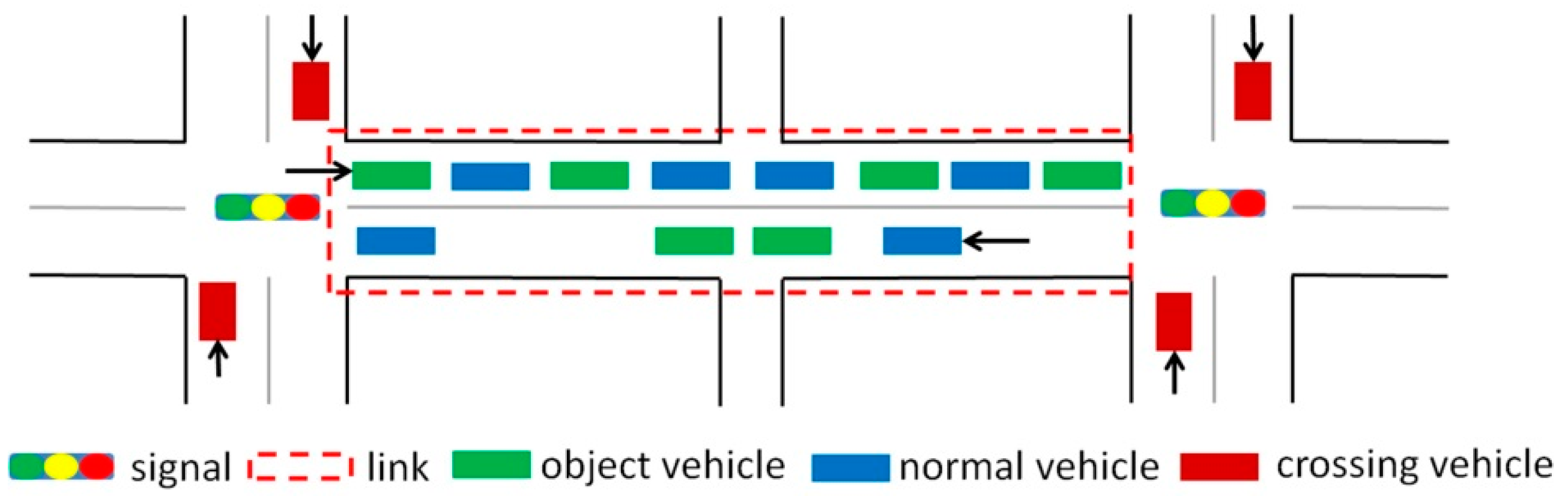
Urban link travel time is influenced by many factors such as signal timing, overtaking behavior, and turning at intersections. In this study, to capture the influence of traffic signals, a link is defined as a segment of the road which is separated by two adjacent signalized intersections. Many researchers have demonstrated that different turning movements experience different delays at signalized intersections and exhibit significantly different distributions [
6]. For simplicity, attention was focused on predicting the travel time for vehicles going straight because vehicles turning left or right from the opposing direction must give way to vehicles going straight, which usually form the majority of the total traffic [
29]. Moreover, in this study, it was assumed that there is a right-turn lane (in the case of Japan) so vehicles going straight were not influenced by vehicles with other turning choices. Because vehicles going straight have priority when going through non-signalized intersections, roads separated by non-signalized intersections were treated as one link with signalized intersections at its endpoints. The link travel time consists of both the time taken to traverse the link and the stopping time due to the traffic and the traffic signal at the downstream intersection. Hence, the exit time of a link was used as the time stamp. For clarity, the main terms in this study are defined in
Table 1 and illustrated in
Figure 1.
There are two main applications of the proposed model in the real world: travel time reliability analysis and reliable route searching. The prediction in the proposed model is represented by a distribution instead of the weighted summation. Travel time distribution can provide more information than the weighted summation such as the travel time variability which plays an important role in travel time reliability measurements. The proposed model can make dynamic link travel time predictions in the form of distribution and these predictions can be used as the input for reliability analysis models such as the mean-variance model [
30,
31]. Li et al. [
31] pointed out that risk-averse travelers are willing to pay for the reduction in travel time variability rather than travel time savings. Some of them prefer the more reliable route, even though the expected travel time is higher in comparison to other routes with shorter expected travel time and higher uncertainty. Chen et al. [
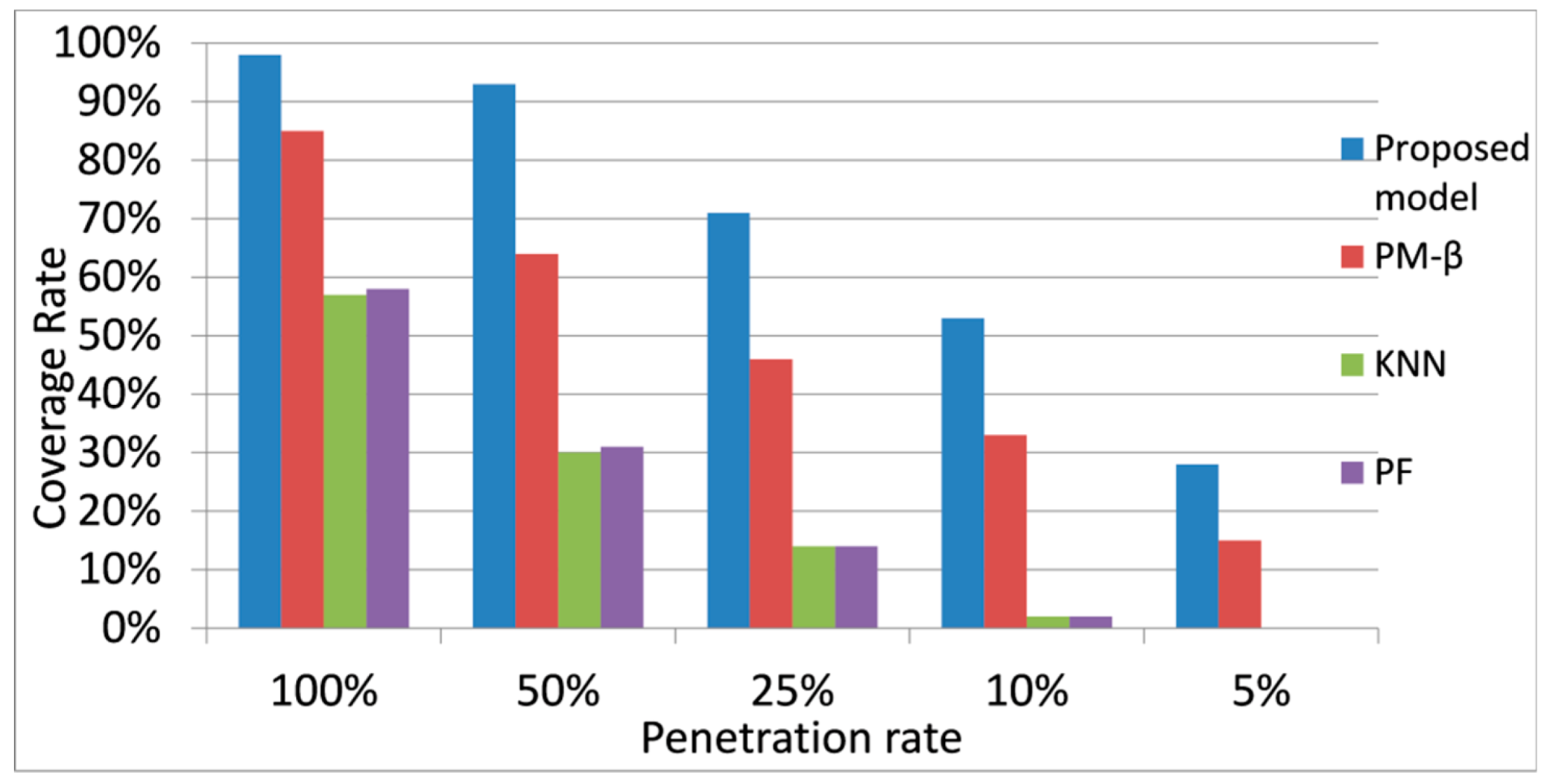
32] proposed a two-stage reliable path-finding algorithm and compared it with other algorithms on the urban network in Wuhan, China. They used the link travel time distributions which were estimated by existing data from a floating-car system as the input of the reliable path-finding algorithms. Because our proposed model could achieve a high coverage rate on urban networks when the penetration rate is low in the real world, its predictions of link travel time distributions can be used for real-time reliable route searching by different reliable path-finding algorithms [
32]. When generating the route travel time, both link travel time and travel time covariance are summed up. In this study, the focus was limited on the link travel time prediction, so the travel time covariance estimation remains as future work.
3.2. Details of the Proposed Model
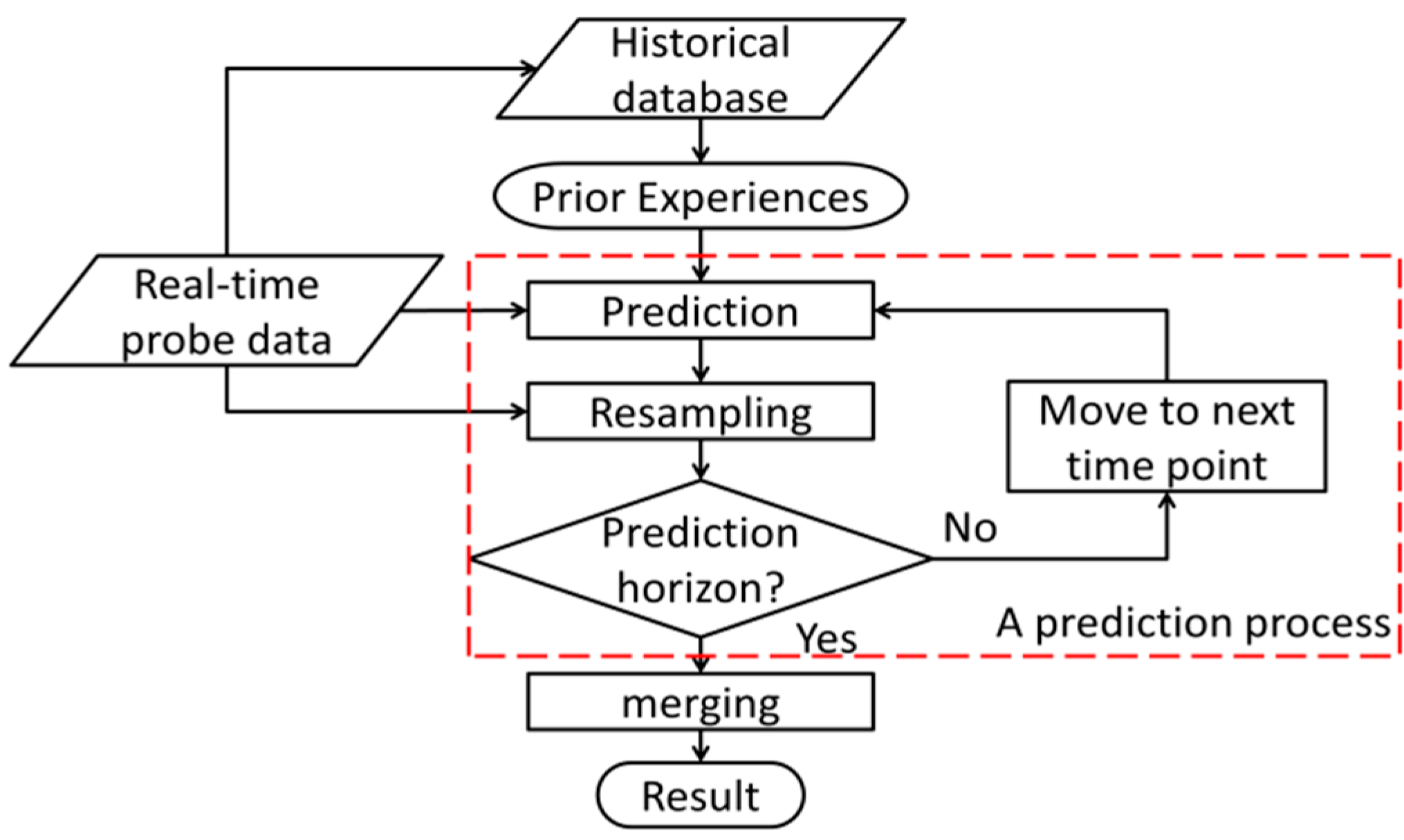
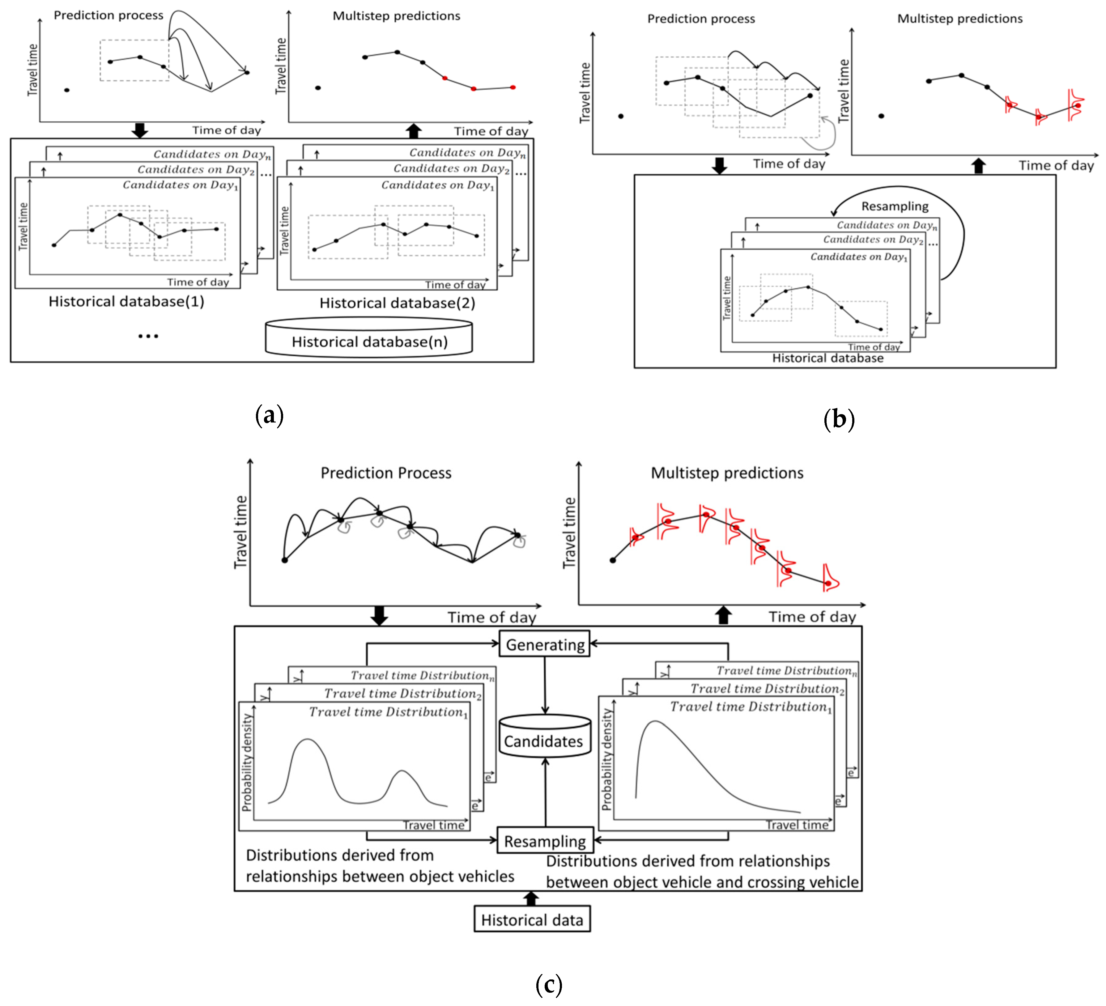
The framework of our proposed model is shown in
Figure 2. The proposed model is based on the prediction process consisting of prediction and resampling. According to Bucknell and Herrera [
5], there is not much difference in prediction when the time interval is shorter than 5 s. In this study, the prediction time interval was set to 5 s so as to capture the frequent changes in travel time on urban networks.
The proposed model can make successive predictions as long as the computation resources are available, which means it is able to make predictions for several minutes or even hours later. However, to reflect the influence of signal timing, the prediction period is based on the average length of the green-light signal phase. Although information about signal timing might be accessible to researchers or even the public in the future, at present, it is still difficult to access in some countries such as Japan. Several methods which use trajectory data from probe vehicles have been developed to estimate signal timing [
33,
34,
35,
36]. However, in this study, there were no trajectory data available before the vehicles stop, so a simple algorithm was developed to approximately estimate the signal timing using the data collected when vehicles exit a link. This algorithm can also be applied to estimate the actuated traffic signal by data from links with similar characteristics and traffic conditions. Details of the estimation algorithm are given in the
Appendix A.
For one prediction, travel time is determined by both the first observed object vehicle’s travel time and the previous travel time prediction. Provided the prediction process starts when there is an observed data
at time point
n, the probability of travel time
at time point
(n + l) can be calculated by
where
represents the probability of travel time
at time point
p given travel time
at time point
q (
) and
is the leaving time difference (LTD) between
p and
q. Parameter
is defined as
, which states that the object vehicle receives more influence from a vehicle that is closer to it. Next, one of the travel time candidates at time point (
n + l) is calculated based on the first
k possible travel times with the biggest probability using
where
is an error term which follows a standard Gaussian distribution. To compare the proposed method with the kNN-based model, a weighted summation of these candidates is used to represent the prediction and weight
is calculated by
where
is the observed travel time and
is a likelihood function, which is chosen to be a standard Gaussian distribution.
Algorithm 1 was proposed for predicting the travel time. The prediction horizon is defined to be the estimated green phase length
MG (
MG=
Length of green phase/5), so each prediction process may have a different length (Line 1). The prediction process starts when an object vehicle is observed (Line 2). If there is more than one object vehicle observed at the same time point, the average travel time is used because the travel times are similar within 5 s in most cases. Here, 100 candidates are generated according to probability
with the corresponding weight
(Lines 3–6). Following that, candidates at step
l are calculated (Lines 7–12). During the prediction, if a new object vehicle is observed at time point (
n + l), a resampling process begins, and the weights are updated (Lines 13–15). If a crossing vehicle is found and it is the first crossing vehicle in the same red phase, the travel time candidate is increased by the length of a red phase
MR (
MR=
Length of red phase/5) because it is assumed that the vehicle must come to a full stop to wait for the signal at the intersection (Line 19–21). Otherwise, the lengths of the candidates remain the same as those at the earlier step if a crossing vehicle is observed (Line 16–18). Moreover, if no new object vehicle is observed, the weights remain the same as that of the preceding step (Lines 22,23).
| Algorithm 1. Proposed Travel Time Prediction Process. |
| 1: | Initialize prediction horizon using Algorithm 3 |
| 2: | If at time point n, there is an observed travel time then |
| 3: | For i = 1:100 do |
| 4: | Generate possible candidate using with error term ; |
| 5: | Calculate similarity for each candidate using (3); |
| 6: | End For |
| 7: | For l = 1: do |
| 8: | For i = 1:100 do |
| 9: | For each possible travel time , calculate probability |
| 10: | at time point (n + l) using (1); |
| 11: | Calculate travel time candidate using (2); |
| 12: | End For |
| 13: | If object vehicle is observed at time point (n + l) then |
| 14: | ; |
| 15: | Begin the resampling process to modify the candidates. |
| 16: | Else if a crossing vehicle is observed at time point (n + l) then |
| 17: | If there is an observed crossing vehicle at time point (n + l − p) then |
| 18: | (l-p < , p < l); |
| 19: | Else |
| 20: | ; |
| 21: | End If |
| 22: | ; |
| 23: | Else, ; |
| 24: | End If |
| 25: | End For |
| 26: | End If |
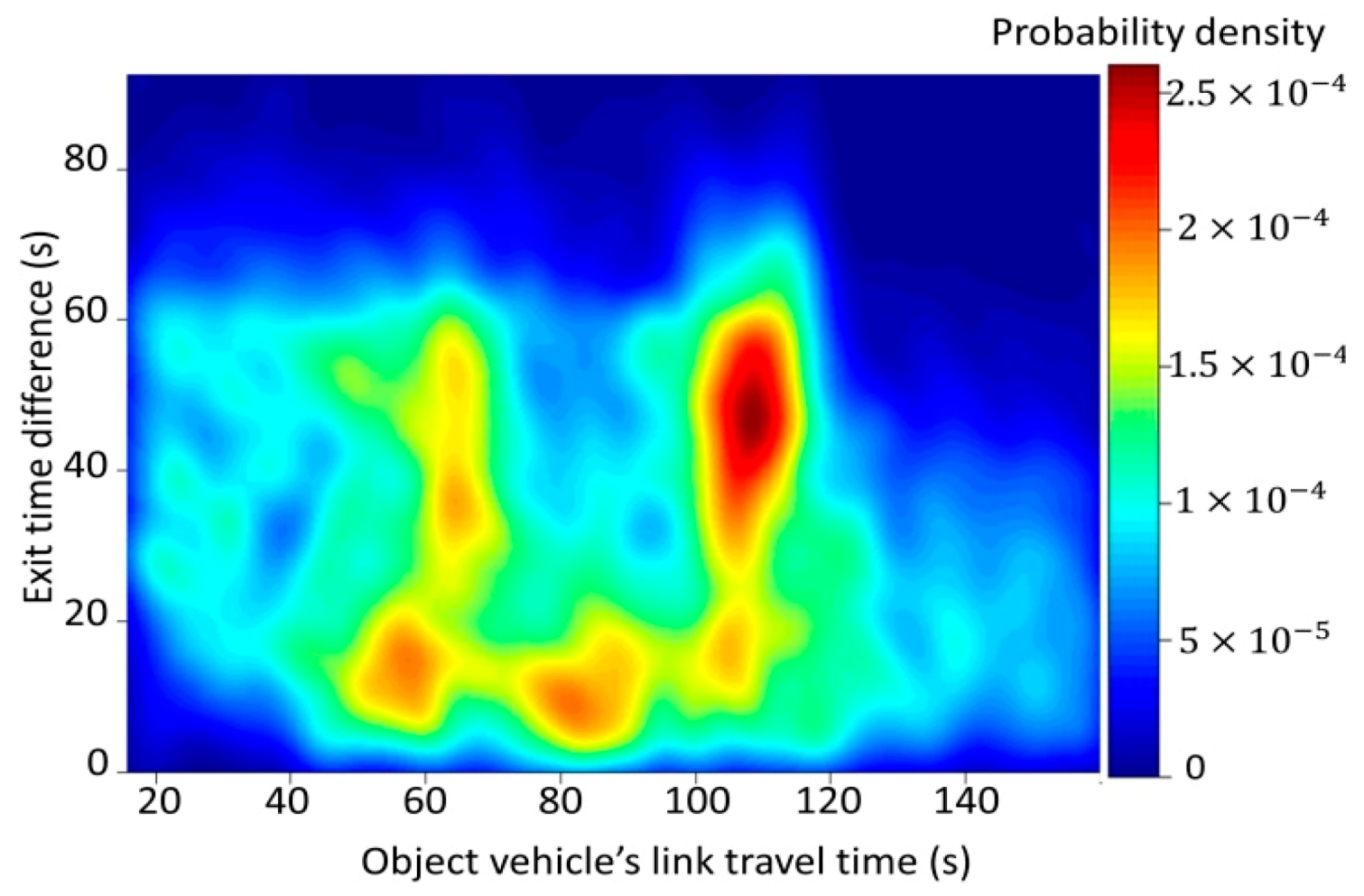
If there is no observed object vehicle, Algorithm 1 cannot be applied, and this situation often happens because of the low penetration rate. To address this situation, an object vehicle’s travel time can be estimated using the travel time distribution under the corresponding exit time difference (ETD) . The ETD is defined as the difference between the exit time of an object vehicle and the last observed crossing vehicle that goes through the intersection before it.
To be specific, the 100 candidates are generated according to the conditional probability . An error term is also added to reflect some unexpected situations. The average travel time of the 100 candidates is used as the object vehicle’s travel time . Given and 100 candidates at time point n, Algorithm 1 can be applied.
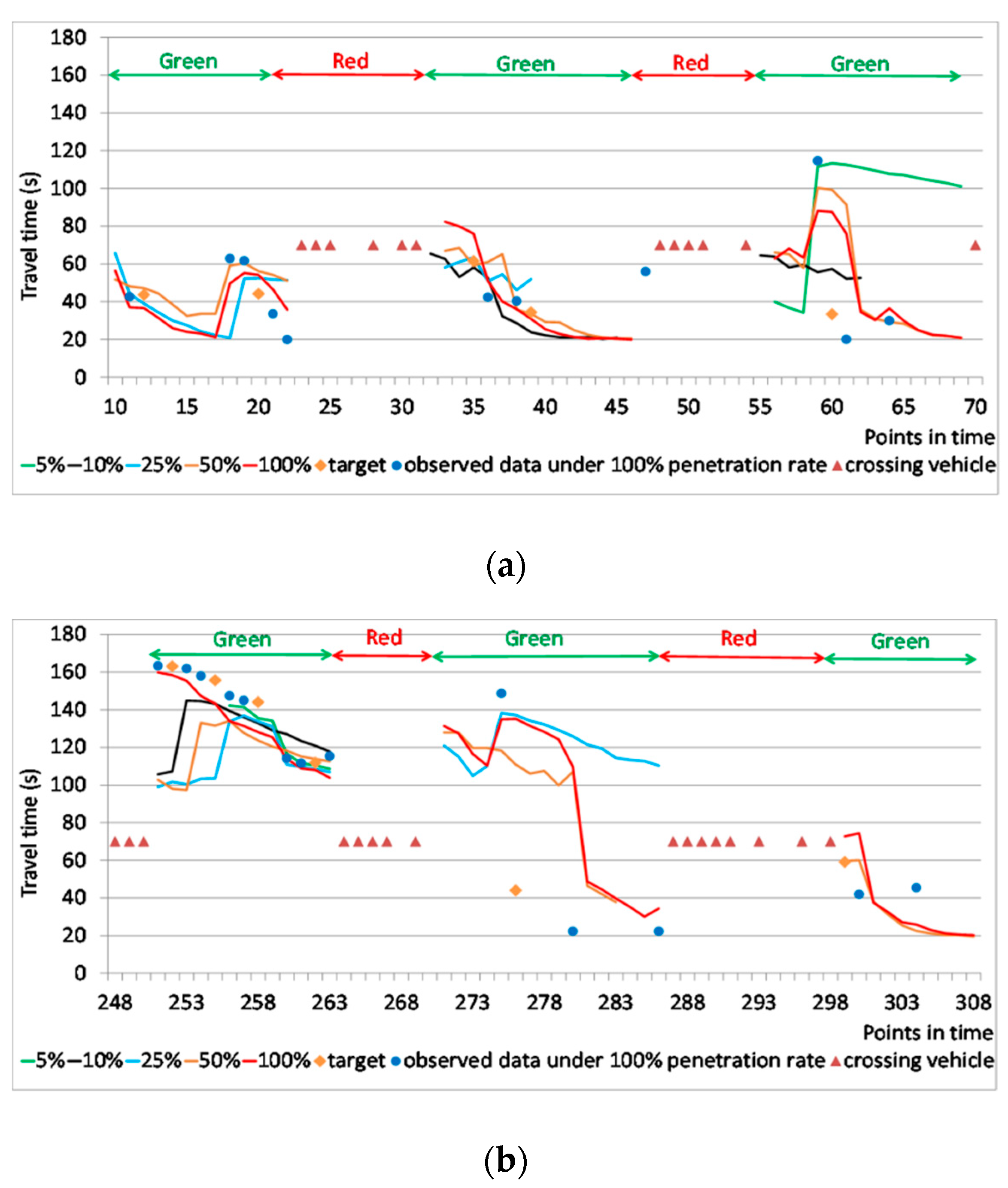
The prediction process tends to decrease the travel time because, in the green phase, the queue is decreasing. Although the travel time might be long at the beginning, it will soon drop to a normal level after several prediction steps. However, when congestion or accidents happen, the queue exists for longer, so the prediction is shorter than the real travel time. The resampling process relieves this problem by replacing candidates with smaller weights with candidates with bigger weights, just as in the conventional PF model. During the prediction process, if a new object vehicle is observed, it will be used to resample candidates at the current step. For example, if the real-time traffic condition is congested, the short travel-time candidates will be replaced by long travel-time candidates. However, this method lacks diversity because it resamples from existing candidates. To improve the diversity, candidates derived from probability are introduced.
Algorithm 2 was proposed for resampling samples. Here, the resampling rate is set to 50%. Providing the resampling process starts at time point
m, the 50 candidates with the lowest weights are removed (Lines 1–3). If the ETD is less than the length of the green phase, another 100 candidates are selected according to conditional probability
and their weights are calculated by (3) (Lines 4–6). Then, new candidates whose weights are bigger than
are added to
(Lines 7–14). If the size of the new candidate set is larger than 100, the candidates with the smallest weight are removed (Line 15–17). Otherwise, candidates are copied randomly until the size increases to 100 (Lines 18–21).
| Algorithm 2 Resampling. |
| 1: | If at time point m, an object vehicle data is observed then |
| 2: | Sort candidates according to their weight in decreasing order, |
| 3: | and remove the later 50 candidates; |
| 4: | If at time point m then |
| 5: | For j = 1:100 do |
| 6: | Select according to , calculate weight using (3); |
| 7: | If then |
| 8: | (k = 1…K); |
| 9: | End If |
| 10: | End For |
| 11: | Combine with |
| 12: | and sort candidates according to weight in decreasing order; |
| 13: | Else K = 0; |
| 14: | End If |
| 15: | If 50 + K > 100 then |
| 16: | Remove the later (K − 50) candidates; |
| 17: | End If |
| 18: | If 50 + K < 100 then |
| 19: | Select (50−K) candidates randomly from |
| 20: | according to their weight and add them to ; |
| 21: | End If |
| 22: | End If |
Because a prediction starts whenever there is an observed object vehicle or an estimated one and the process continues until it reaches the prediction horizon, there might be several predictions for the same time point. Therefore, it is necessary to merge these predictions into one. The candidates from each prediction are determined. The number of candidates is proportional to the duration between the starting and merging time points. The weight of each selected candidate is normalized, and then either a weighted summation or the candidate with the maximum weight is used to compare with the prediction results of the kNN-based and the PF-based models.


