Analysis of a Tubular Torsionally Resonating Viscosity–Density Sensor


Abstract
:1. Introduction
2. Sensor Design and Experiments
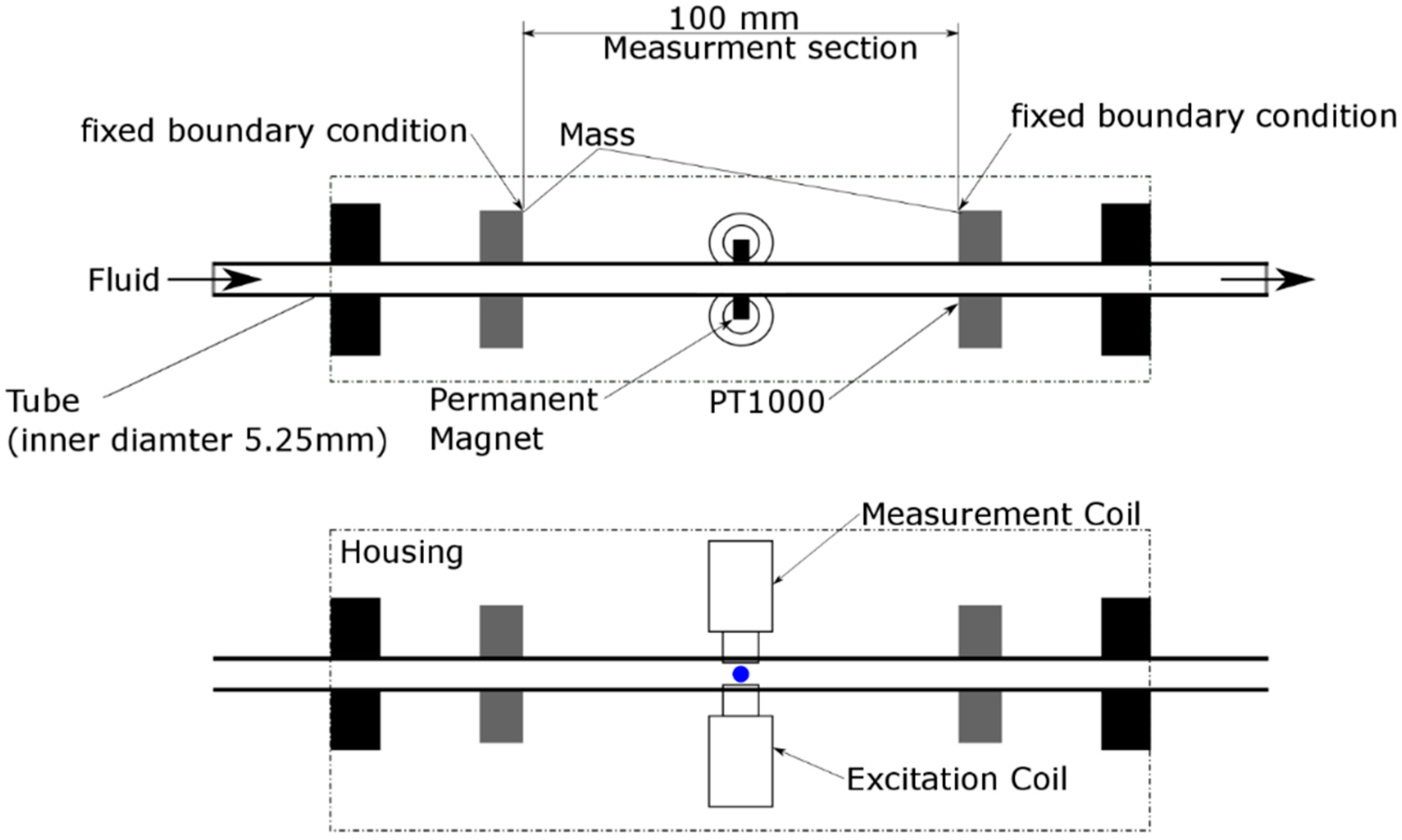
2.1. Tubular Sensor Design
2.2. Static Experiment Procedure
- (1)
- An absolute error in the measured damping was caused by the intrinsic damping of the sensor. This error was independent of the damping value.
- (2)
- Measurement of the damping value was more accurate at low damping due to higher signal-to-noise ratio. The relative error was 0.3% in air and increased to 30% for viscosities of 1000 mPas at a density of 1000 kg/m³. This error could be reduced by averaging multiple measurements. Thus, by averaging 100 measurements, its contribution was reduced by ten-fold.
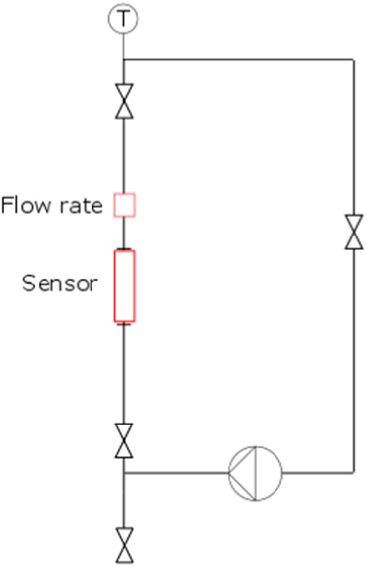
2.3. Flow Loop Experiment
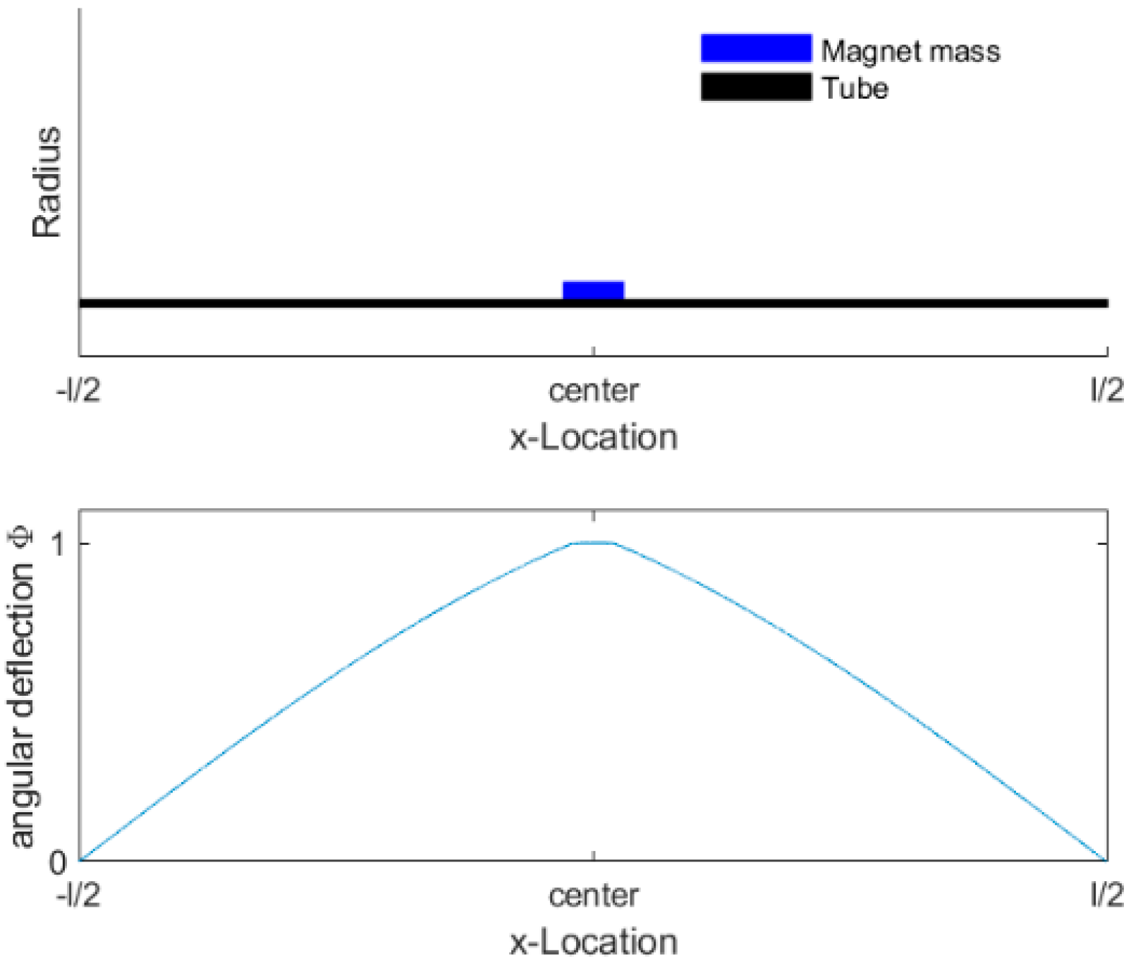
2.4. Resonator Modeling
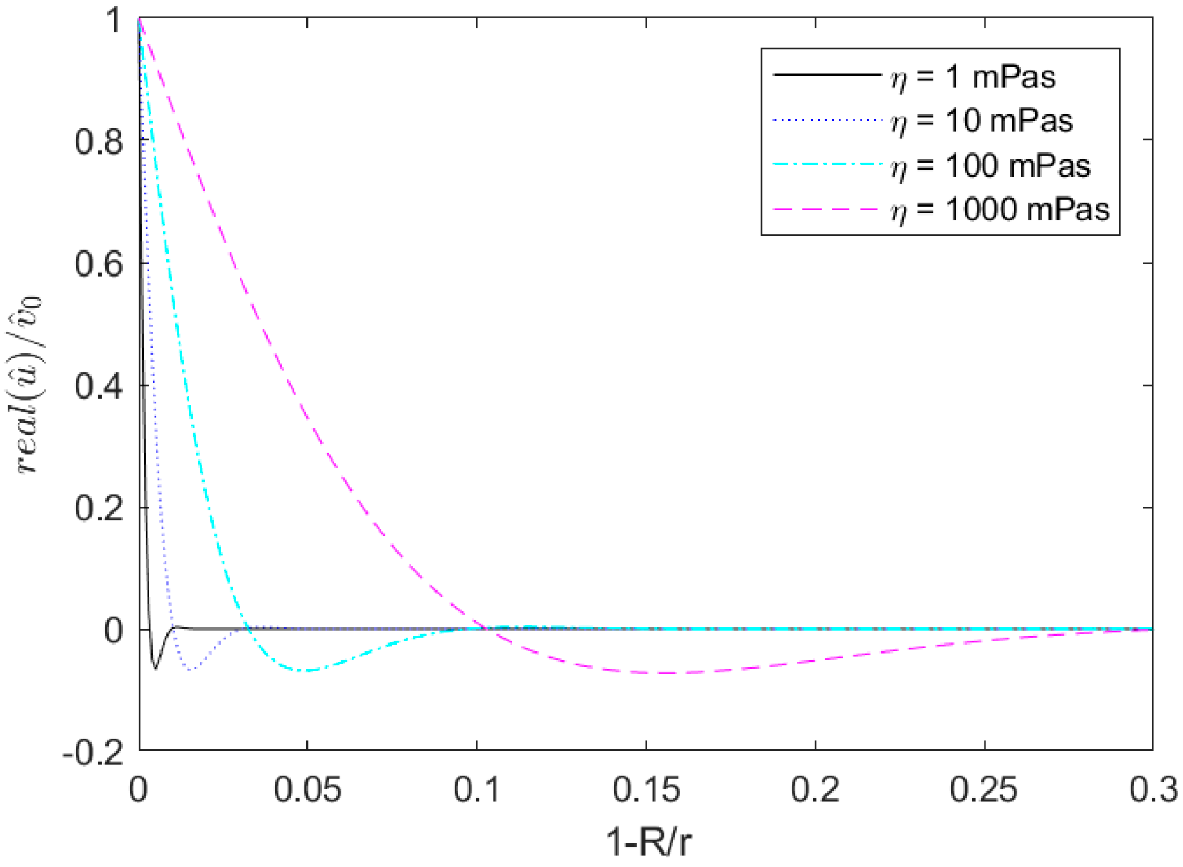
Fluid Forces
3. Discussion
3.1. Static Flow Conditions
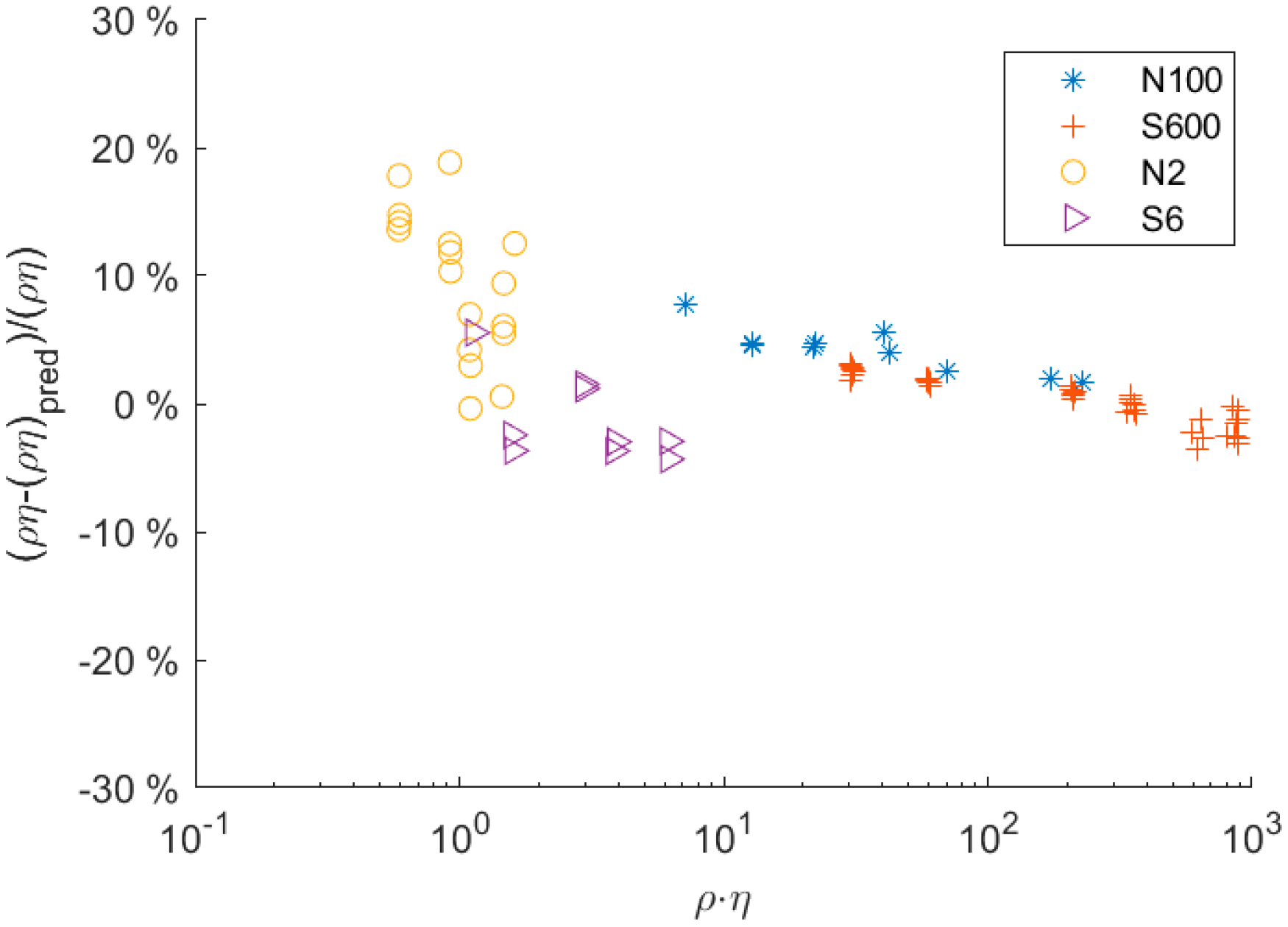
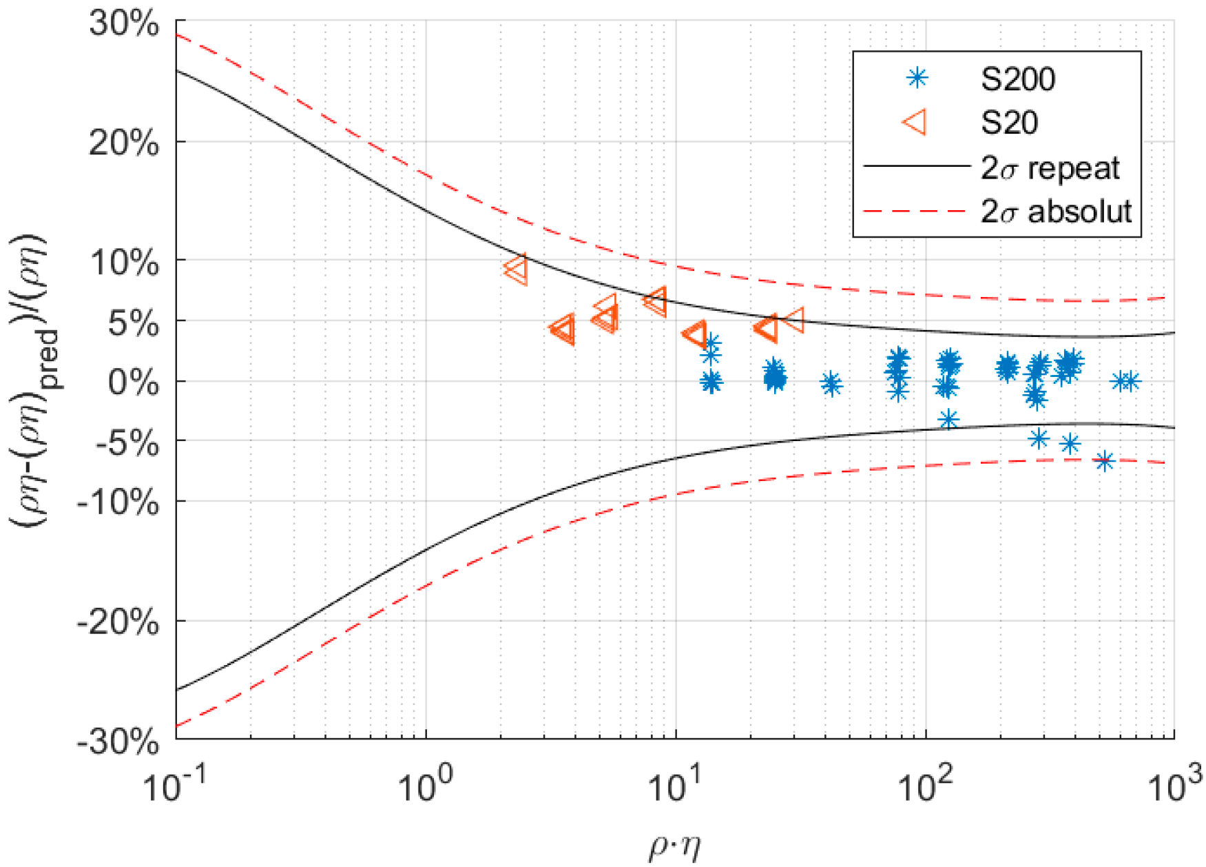
- (1)
- Bias in the damping measurement: At high damping, the signal-to-noise ratio (SNR) decreased due to the smaller amplitude of the resonator. The algorithm used to determine the damping was sensitive to the noise in the signal. As the SNR decreased, the error in the evaluation of the damping value increased. The error is not normally distributed but had a bias towards smaller damping values. Hence, the evaluated averaged value of the damping tended to be underpredicted as the SNR decreased. This behavior could be qualitatively simulated and showed a similar trend, as was experimentally observed.
- (2)
- Distortion of modal function: Another potential source of the systematic deviation is the fluid–structure interactions. At high values, the fluid exerts forces on the tube that are much higher than those exerted at low values; thus, the balance between structural and fluid forces changes. In the model, the modal shape was computed under the assumption that the fluid forces did not impact the shape of the mode. Hence, this assumption may no longer be valid for fluids with high values. To account for and verify this effect, the fluid–structure interaction (strong coupling) will be incorporated into the numerical model in future studies. This would allow specific investigation of the impact of fluid properties on the structural mode and its implications at values.
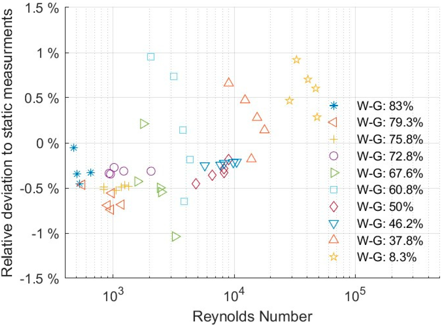
3.2. Flow Loop
4. Conclusions
Author Contributions
Funding
Acknowledgments
Conflicts of Interest
References
- Papi, M.; Maulucci, G.; Arcovito, G.; Paoletti, P.; Vassalli, M.; De Spirito, M. Detection of Microviscosity by Using Uncalibrated Atomic Force Microscopy Cantilevers. Appl. Phys. Lett. 2008, 93, 4102. [Google Scholar] [CrossRef]
- Ghatkesar, M.K.; Braun, T.; Barwich, V.; Ramseyer, J.P.; Gerber, C.; Hegner, M.; Lang, H.P. Resonating Modes of Vibrating Microcantilevers in Liquid. Appl. Phys. Lett. 2008, 92, 10–13. [Google Scholar] [CrossRef] [Green Version]
- Papi, M.; Arcovito, G.; De Spirito, M.; Vassalli, M.; Tiribilli, B. Fluid viscosity determination by means of uncalibrated atomic force microscopy cantilevers. Appl. Phys. Lett. 2006, 88, 194102. [Google Scholar] [CrossRef] [Green Version]
- Shih, W.Y.; Li, X.; Gu, H.; Shih, W.-H.; Aksay, I.A. Simultaneous liquid viscosity and density determination with piezoelectric unimorph cantilevers. J. Appl. Phys. 2001, 89, 1497–1505. [Google Scholar] [CrossRef] [Green Version]
- McLoughlin, N.; Lee, S.; Hähner, G. Simultaneous determination of density and viscosity of liquids based on resonance curves of uncalibrated microcantilevers. Appl. Phys. Lett. 2006, 89, 184106. [Google Scholar] [CrossRef]
- Thompson, M.; Kipling, A.L.; Duncan-Hewitt, W.C.; Rajakovi?, L.V.; Avi-Vlasak, B.A.; Rajaković, L.V.; Cavic-Vlasak, B.A. Thickness-shear-mode acoustic wave sensors in the liquid phase. A review. Analyst 1991, 116, 881–890. [Google Scholar] [CrossRef]
- Tessier, L.; Patat, F.; Schmitt, N.; Feuillard, G.; Thompson, M. Effect of the Generation of Compressional Waves on the Response of the Thickness-Shear Mode Acoustic Wave Sensor in Liquids. Anal. Chem. 1994, 66, 3569–3574. [Google Scholar] [CrossRef]
- Keiji Kanazawa, K.; Gordon, J.G. The Oscillation Frequency of a Quartz Resonator in Contact with Liquid. Anal. Chim. Acta 1985, 175, 99–105. [Google Scholar] [CrossRef]
- Huang, L.; Chen, J.; Cao, T.; Cong, H.; Cao, W. Investigation of Microtribological Properties of C60-Containing Polymer Thin Films Using AFM/FFM. Wear 2003, 255, 826–831. [Google Scholar] [CrossRef]
- Kim, S.; Lee, D.; Yun, M.; Jung, N.; Jeon, S.; Thundat, T. Multi-Modal Characterization of Nanogram Amounts of a Photosensitive Polymer. Appl. Phys. Lett. 2013, 102, 2–6. [Google Scholar] [CrossRef] [Green Version]
- Bistac, S.; Schmitt, M.; Ghorbal, A.; Gnecco, E.; Meyer, E. Nano-Scale Friction of Polystyrene in Air and in Vacuum. Polymer 2008, 49, 3780–3784. [Google Scholar] [CrossRef]
- Martin, F.; Newton, M.I.; McHale, G.; Melzak, K.A.; Gizeli, E. Pulse Mode Shear Horizontal-Surface Acoustic Wave (SH-SAW) System for Liquid Based Sensing Applications. Biosens. Bioelectron 2004, 19, 627–632. [Google Scholar] [CrossRef]
- Voinova, M.V.; Rodahl, M.; Jonson, M.; Kasemo, B. Viscoelastic Acoustic Response of Layered Polymer Films at Fluid-Solid Interfaces: Continuum Mechanics Approach. Phys. Scripta. 1998, 59, 391–396. [Google Scholar] [CrossRef] [Green Version]
- Lucklum, R.; Behling, C.; Cernosek, R.W.; Martin, S.J. Determination of Complex Shear Modulus with Thickness Shear Mode Resonators. J. Phys. D. Appl. Phys. 1997, 30, 346–356. [Google Scholar] [CrossRef]
- Xie, J.; Hu, Y. A Two-Dimensional Model on the Coupling Thickness-Shear Vibrations of a Quartz Crystal Resonator Loaded by an Array Spherical-Cap Viscoelastic Material Units. Ultrasonics 2016, 71, 194–198. [Google Scholar] [CrossRef]
- Dohn, S.; Hansen, O.; Boisen, A. Cantilever Based Mass Sensor with Hard Contact Readout. Appl. Phys. Lett. 2006, 88, 1–4. [Google Scholar] [CrossRef] [Green Version]
- Lang, H.P.; Hegner, M.; Gerber, C. Cantilever Array Sensors. Nanobiotechnol. II More Concepts Appl. 2007, 8, 175–195. [Google Scholar] [CrossRef]
- Datar, R.; Passian, A.; Desikan, R.; Thundat, T. Microcantilever Biosensors. Proc. IEEE Sens. 2007, 37, 5. [Google Scholar] [CrossRef]
- Stachiv, I.; Fedorchenko, A.I.; Chen, Y.-L. Mass Detection by Means of the Vibrating Nanomechanical Resonators. Appl. Phys. Lett. 2012, 100, 093110. [Google Scholar] [CrossRef]
- Qin, L.; Cheng, H.; Li, J.M.; Wang, Q.M. Characterization of Polymer Nanocomposite Films Using Quartz Thickness Shear Mode (TSM) Acoustic Wave Sensor. Sens. Actuators A Phys. 2007, 136, 111–117. [Google Scholar] [CrossRef]
- Brack, T. Multi-Frequency Phase Control of a Torsional Oscillator for Applications in Dynamic Fluid Sensing. Ph.D. Thesis, ETH Zurich, Zurich, Swizerland, 2017. [Google Scholar]
- Brack, T.; Dual, J. Multimodal torsional vibrations for the characterization of complex fluids. In WIT Transactions on the Built Environment; Computational Mechanics WIT Press: Southampton, UK, 2013; Volume 129, pp. 191–199. [Google Scholar] [CrossRef]
- Brack, T.; Bolisetty, S.; Dual, J. Simultaneous and Continuous Measurement of Shear Elasticity and Viscosity of Liquids at Multiple Discrete Frequencies. Rheol. Acta 2018, 57, 415–428. [Google Scholar] [CrossRef]
- Valtorta, D.; Mazza, E. Dynamic Measurement of Soft Tissue Viscoelastic Properties with a Torsional Resonator Device. Med. Image Anal. 2005, 9, 481–490. [Google Scholar] [CrossRef] [PubMed]
- Dual, J. Experimental Methods in Wave Propagationin Solids and Dynamic Viscometry. Ph.D. Thesis, ETH Zurich, Zurich, Swizerland, 1989. [Google Scholar]
- Reinhart, W.H.; Hausler, K.; Schaller, P.; Erhart, S.; Stetter, M.; Dual, J.; Sayir, M. Rheological Properties of Blood as Assessed with a Newly Designed Oscillating Viscometer. Clin. Hemorheol Microcirc. 1998, 18, 59–65. [Google Scholar] [PubMed]
- Brunner, D.; Khawaja, H.; Moatamedi, M.; Boiger, G. CFD modelling of pressure and shear rate in torsionally vibrating structures using ANSYS CFX and COMSOL multiphysics. Int. J. Multiphysics 2018, 12, 349–358. [Google Scholar]
- Clara, S.; Feichtinger, F.; Voglhuber-Brunnmaier, T.; Niedermayer, A.O.; Tröls, A.; Jakoby, B. Balanced Torsionally Oscillating Pipe Used as a Viscosity Sensor. Meas. Sci. Technol. 2019, 30. [Google Scholar] [CrossRef]
- Clara, S.; Antlinger, H.; Feichtinger, F.; Niedermayer, A.O.; Voglhuber-Brunnmaier, T.; Jakoby, B. A balanced flow-through viscosity sensor based on a torsionally resonating pipe. Proc. IEEE Sens. 2017, 1–3. [Google Scholar] [CrossRef]
- Häusler, K.; Reinhart, W.H.; Schaller, P.; Dual, J.; Goodbread, J.; Sayir, M. A newly designed oscillating viscometer for blood viscosity measurements. Biorheology 1996, 33, 397–404. [Google Scholar] [CrossRef]
- Fuchs, M.; Drahm, W.; Matt, C.; Wenger, A. A coriolis meter with direct viscosity measurement. Comput. Control. Eng. J. 2003, 14, 42–43. [Google Scholar]
- Kierzenka, J.; Shampine, L.F. A BVP solver based on residual control and the maltab PSE. ACM Trans. Math. Softw. 2001, 27, 299–316. [Google Scholar] [CrossRef]

© 2020 by the authors. Licensee MDPI, Basel, Switzerland. This article is an open access article distributed under the terms and conditions of the Creative Commons Attribution (CC BY) license (http://creativecommons.org/licenses/by/4.0/).
Share and Cite
Brunner, D.; Goodbread, J.; Häusler, K.; Kumar, S.; Boiger, G.; Khawaja, H.A. Analysis of a Tubular Torsionally Resonating Viscosity–Density Sensor. Sensors 2020, 20, 3036. https://doi.org/10.3390/s20113036
Brunner D, Goodbread J, Häusler K, Kumar S, Boiger G, Khawaja HA. Analysis of a Tubular Torsionally Resonating Viscosity–Density Sensor. Sensors. 2020; 20(11):3036. https://doi.org/10.3390/s20113036
Chicago/Turabian StyleBrunner, Daniel, Joe Goodbread, Klaus Häusler, Sunil Kumar, Gernot Boiger, and Hassan A. Khawaja. 2020. "Analysis of a Tubular Torsionally Resonating Viscosity–Density Sensor" Sensors 20, no. 11: 3036. https://doi.org/10.3390/s20113036