A Nondestructive Testing Method for the Determination of the Complex Refractive Index Using Ultra Wideband Radar in Industrial Applications


Abstract
:1. Introduction
2. Theory
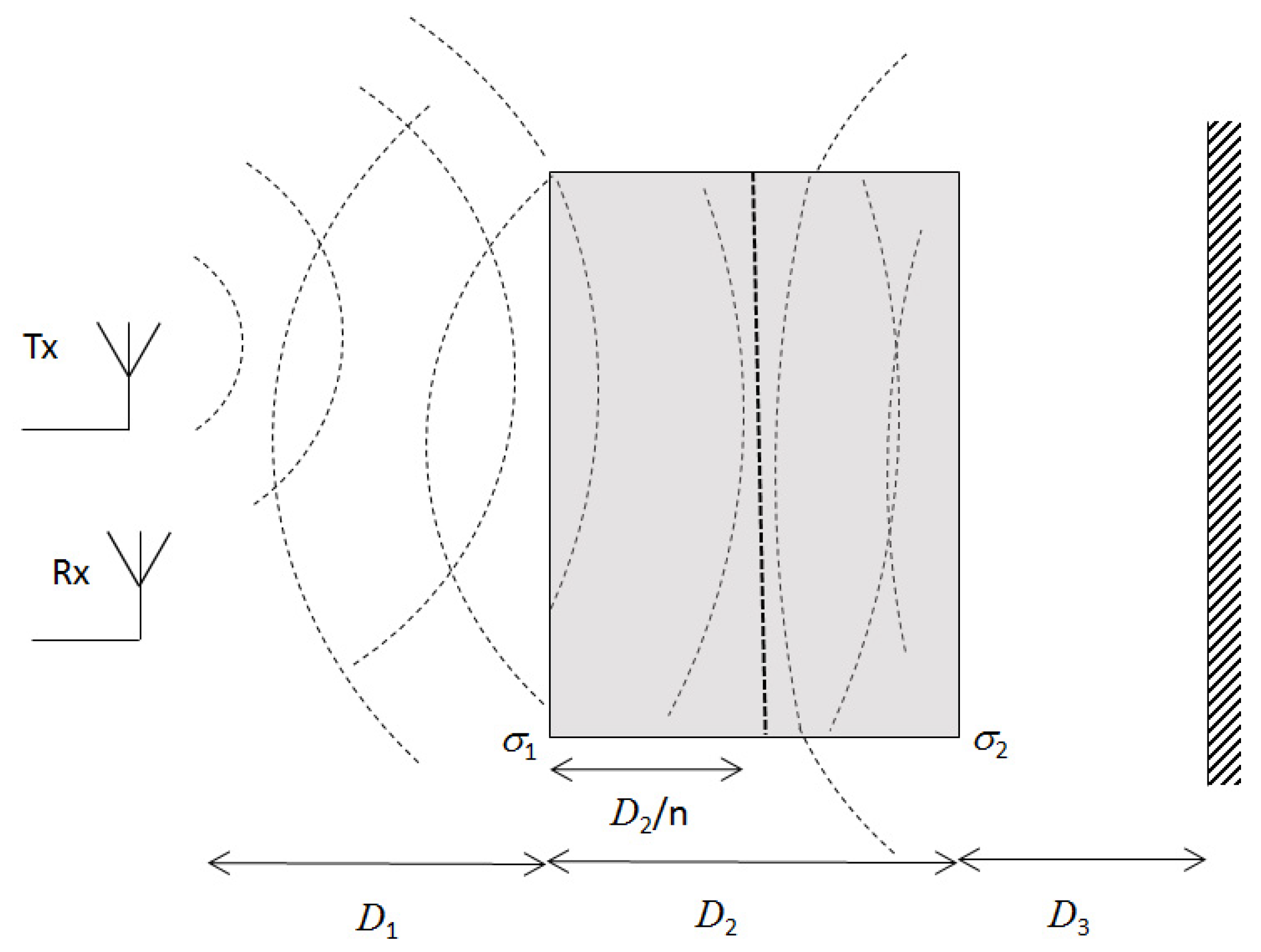
2.1. Wave Propagation Model
2.2. Anisotropy and Polarimetry
2.3. Refractive Index Determination
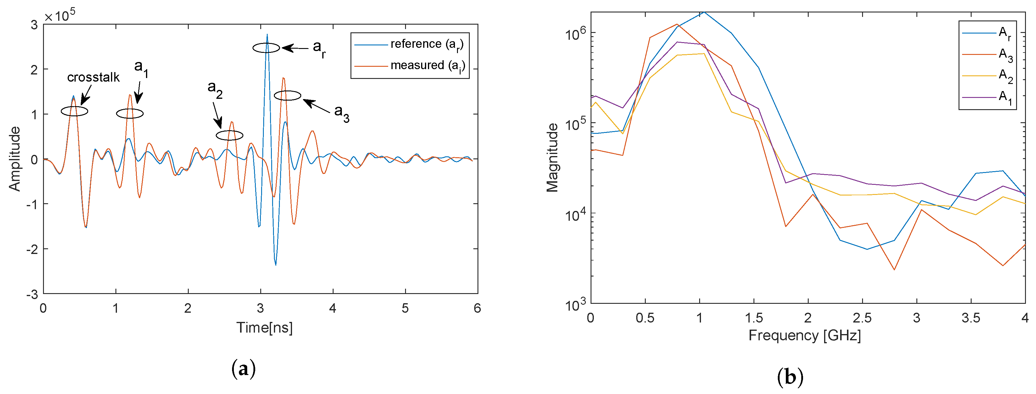
- Find the maximum value and the corresponding time instants of the time series. Define a time interval around this time instant; this is now one pulse.
- Find the maximum value and the corresponding time instant of the time series, without the time interval from Step 1.
- Continue until two () or three () pulses have been detected.
- Sort the pulses in adjacent order in time such that pulse , , and are obtained.
2.4. Error Analysis
3. Experiment
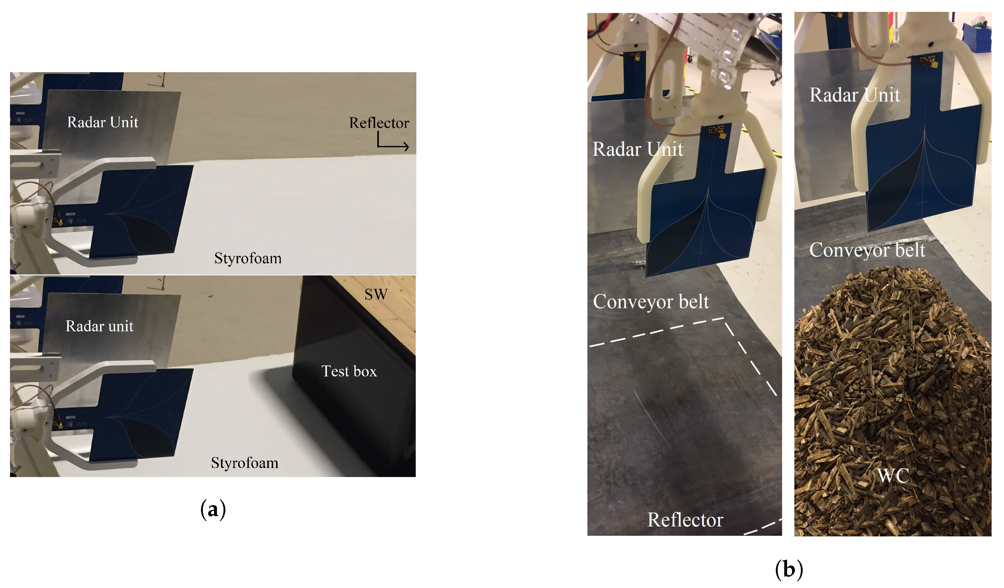
3.1. Radar System and Setup
- The objects were placed horizontally and were illuminated horizontally with a flat reference reflector behind the object. The objects were put 1 m above the ground on Styrofoam blocks (with ) to minimize reflections from the ground surface. This case corresponds to an industrial application, which requires an investigation of dielectric properties of materials contained in boxes or cases with a conveyor belt with, e.g., piles of wood being tested in-line horizontally (Figure 4b). The distance between the object and the reference is arbitrary, but .
- The objects were on a conveyor belt with the radar unit illuminating the samples vertically from above. This case corresponds to an industrial application in which, e.g., wood chips are tested in-line (Figure 4b). In this case, the object is adjacent to the reference, and .
3.2. Objects
- Piles of planks of SW inside the test boxes were used (used in Test Setup I, in Section 3.1):Hard pine wood was cut into small pieces of piles of SW planks to fit in plastic boxes. The dimensions of SW planks were 50–60 mm in width, 20–35 mm in thickness, and 100–400 mm in length. The SW was placed inside the plastic boxes in such a way that the orientation of wood fibers were in one direction, i.e., parallel to the ground, with no spacing in between the SW planks, as shown in Figure 4b. The dimensions of the plastic boxes were 60 cm × 30 cm × 30 cm, and the thickness of the box’s wall was very small (2 mm) compared to the operating wavelength.
- WCs inside test boxes were investigated (used in Test Setup I, in Section 3.1):The WCs were filtered to remove dust or sand before filled into the plastic boxes. The dimensions of the chips were 1.5–20 mm in width/thickness and 22–70 mm in length. The chips were manually distributed inside the box, which gives a random orientation of the WCs in the horizontal plane. Gravity oriented the chips such that an anisotropic medium was obtained [10]. The dimensions and the wall thickness of plastic boxes were the same as above. Note that no external pressure was applied to the WCs inside the box during the filling process.
- Piles of SW planks on the conveyor belt were investigated (used in Test Setup II, in Section 3.1):Piles of planks of SW were placed directly on the conveyor belt. The dimensions of SW were as mentioned above. The arrangement of SW on the conveyor belt was such that the orientation of wood fibers are in one direction, i.e., parallel to the conveyor-belt’s length. In this case, there is no specific geometry of volume of piles of SW planks, but the height is in the range of 30–40 cm. A standard industrial size of the conveyor belt with a width of 2 m, a thickness of 30 mm, and a length limited to 2 m was used.
- WCs on the conveyor belt were used as the last type of object (used in Test Setup II, in Section 3.1):Bark WCs were placed directly on the conveyor belt. The dimensions of the WC were the same as above. WCs were manually distributed on the conveyor-belt in such a way that the orientation of the WCs was random in the horizontal plane, but oriented by gravity to yield an isotropic medium [10]. In this case, there was no specific geometry of the volume of WC samples, but the height was in the range of 20–40 cm. A standard industrial size of conveyor belt with aforementioned dimensions was used.
3.3. System Characterization
- Variation of the distance to the objects, with objects of different size. The objects were metallic sheets of size varying from 10 × 10 cm to 200 × 200 cm. Te distance was varied from 20 to 150 cm.
- Repeatability was tested by 20 consecutive measurements with a metallic sheet of 100–100 cm at a distance of 30 cm.
3.4. Experiment Preparation and Procedure
4. Results
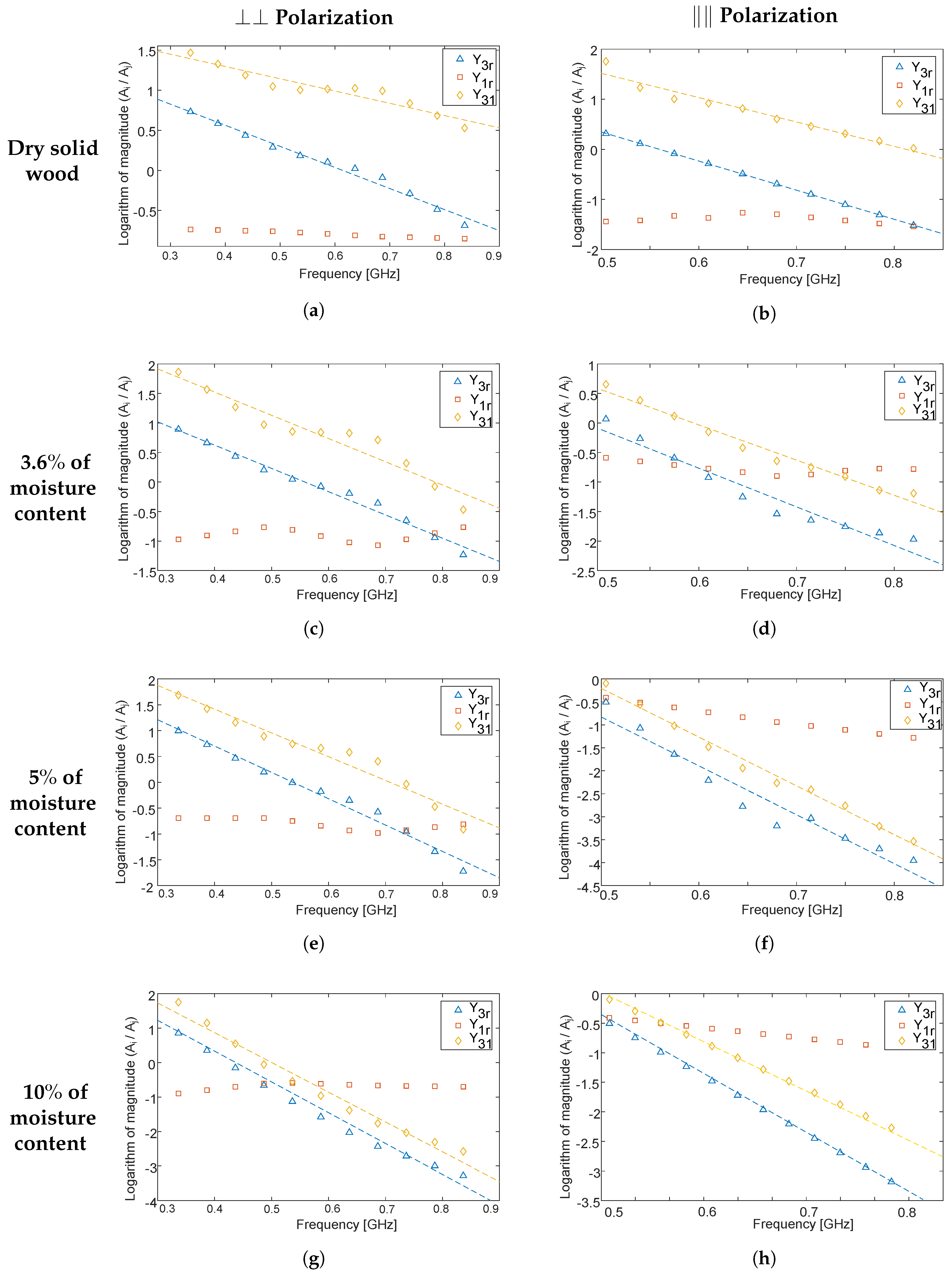
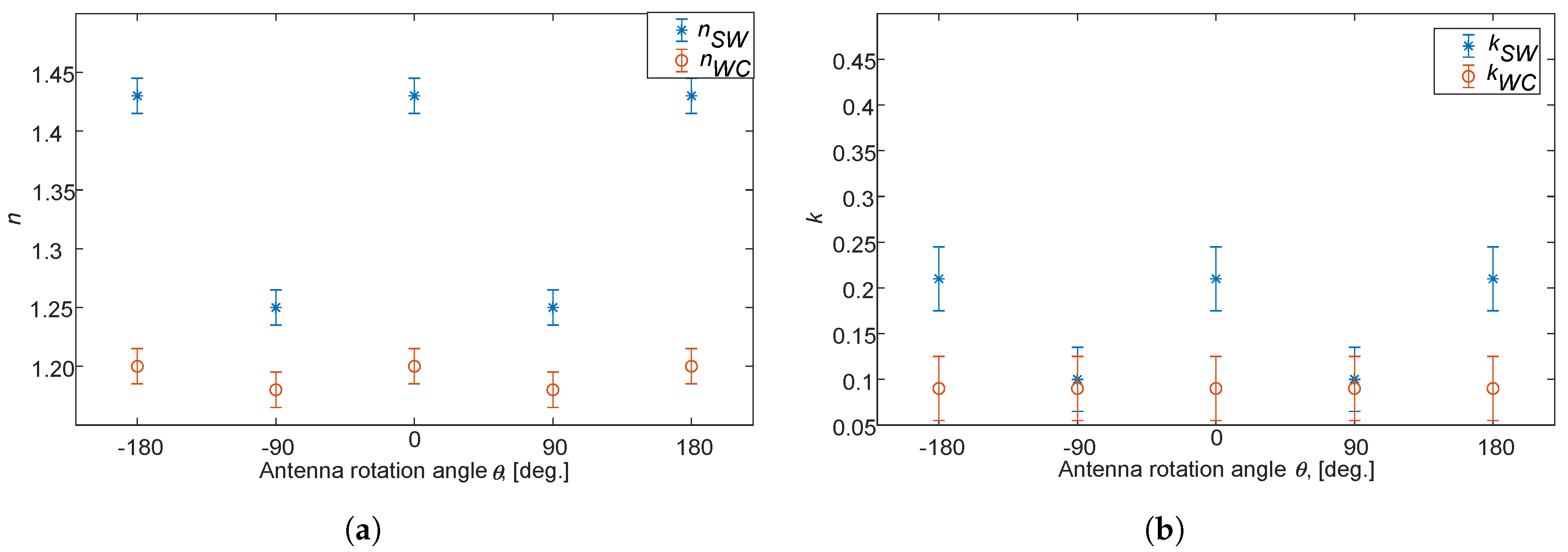
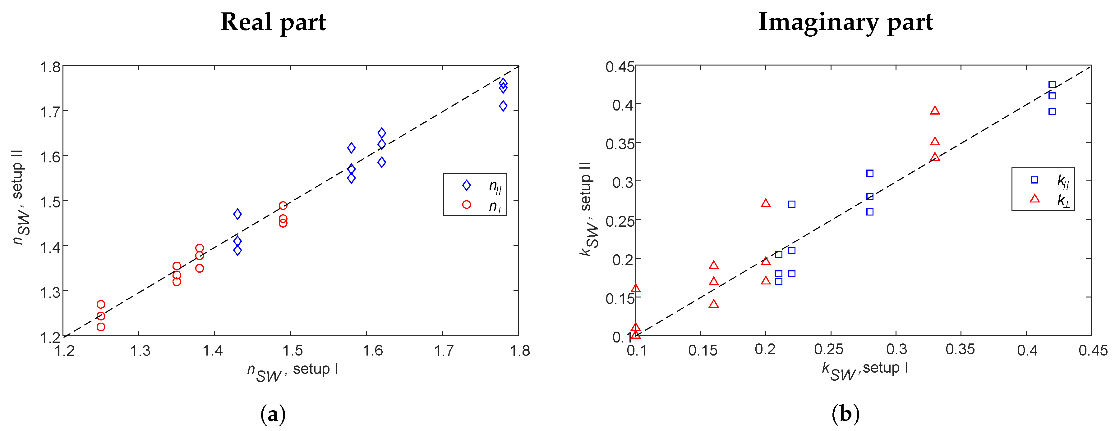
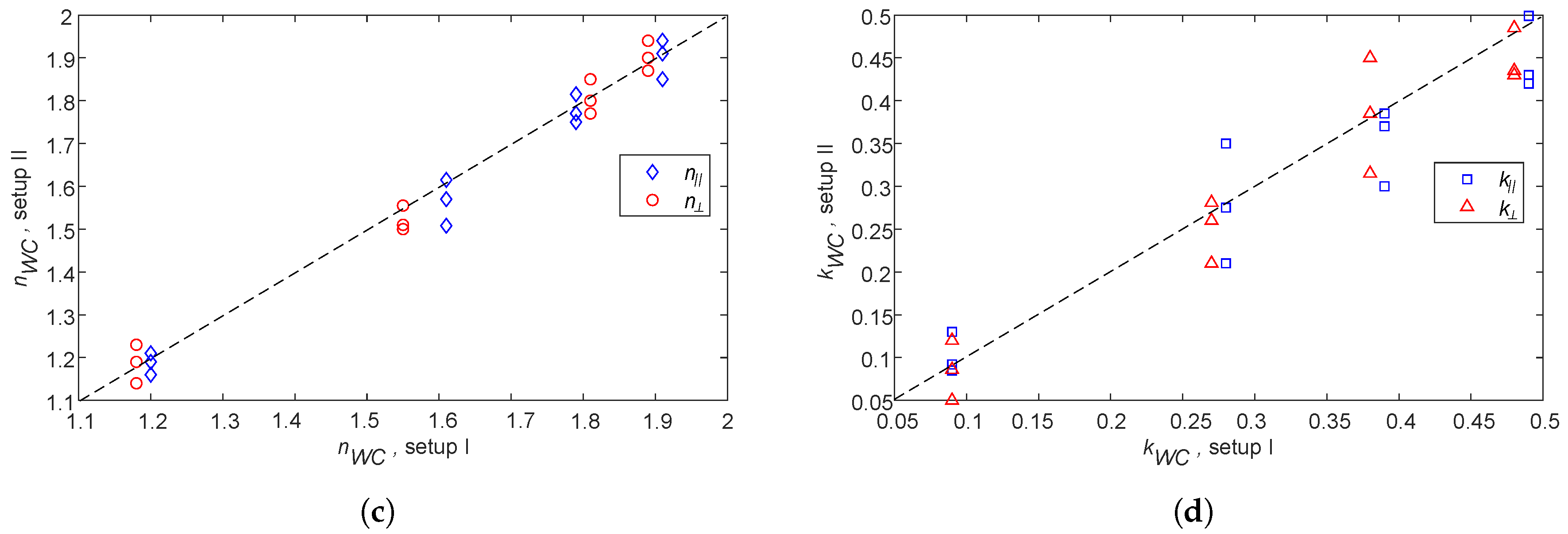
4.1. Boxes
4.2. Conveyor Belt
5. Discussion
6. Conclusions
Author Contributions
Funding
Acknowledgments
Conflicts of Interest
Abbreviations
| EM | Electromagnetic |
| UWB | Ultra Wide Band |
| SW | Solid Wood |
| WCs | Wood Chips |
| RCS | Radar cross section |
References
- Sachs, J. Ultra wide band radar applications and uses. In Handbook of Ultra-Wide band Short-Range Sensing: Theory, Sensors, Applications; Wiley-VCH Verlag and Co. KGaA: Weinheim, Germany, 2012; pp. 363–698. [Google Scholar]
- Kosch, O.; Thiel, F.; Seifert, F.; Sachs, J.; Hein, M.A. Motion detection In-Vivo by multi-channel ultrawideband radar. In Proceedings of the IEEE International Conference on Ultra-Wideband, Syracuse, NY, USA, 17–20 September 2012; pp. 392–396. [Google Scholar]
- Choudhary, V.; Rönnow, D.; Jansson, M. A Singular Value Decomposition Based Approach for Classifying Concealed Objects in Short Range Polarimetric Radar Imaging. In Proceedings of the PhotonIcs & Electromagnetics Research Symposium, Rome, Italy, 17–20 June 2019; pp. 4109–4115. [Google Scholar]
- Zhekov, S.S.; Franek, O.; Pedersen, G.F. Dielectric Properties of Common Building Materials for Ultrawideband Propagation Studies. IEEE Antennas Propag. Mag. 2020, 62, 72–81. [Google Scholar] [CrossRef]
- Dietrich, M.; Rauch, D.; Porch, A.; Moos, R. A laboratory test setup for in situ measurements of the dielectric properties of catalyst powder samples under reaction conditions by microwave cavity perturbation: Set up and initial tests. Sensors 2014, 14, 16856–16868. [Google Scholar] [CrossRef] [PubMed] [Green Version]
- Ramos, A.; Girbau, D.; Lazaro, A.; Villarino, R. Wireless concrete mixture composition sensor based on time-coded UWB RFID. IEEE Microw. Wirel. Compon. Lett. 2015, 25, 681–683. [Google Scholar] [CrossRef]
- Gubinelli, S.; Paolini, E.; Giorgetti, A.; Mazzotti, M.; Rizzo, A.; Troiani, E.; Chiani, M. An ultra-wideband radar approach to nondestructive testing. In Proceedings of the IEEE International Conference on Ultra-WideBand, Paris, France, 1 September 2014; pp. 303–308. [Google Scholar]
- Maunder, A.; Taheri, O.; Fard, M.R.G.; Mousavi, P. Calibrated layer-stripping technique for level and permittivity measurement with UWB radar in metallic tanks. IEEE Trans. Microw. Theory Tech. 2015, 63, 2322–2334. [Google Scholar] [CrossRef]
- Taheri, O.; Maunder, A.; Mousavi, P. Correlation-based UWB radar for thin layer resolution. IEEE Antennas Wirel. Propag. Lett. 2015, 15, 901–904. [Google Scholar] [CrossRef]
- Ottosson, P.; Andersson, D.; Rönnow, D. UWB Radio Measurement and Time-Domain Analysis of Anisotropy in Wood Chips. IEEE Sens. J. 2018, 18, 9112–9119. [Google Scholar] [CrossRef]
- Repko, M.; Gamec, J.; Kurdel, P.; Gamcová, M. Estimation of the Wall Thickness and Relative Permittivity by Radar System. In Proceedings of the 16th International Conference on Emerging eLearning Technologies and Applications, Vysoké Tatry, Slovakia, 15 November 2018; pp. 469–474. [Google Scholar]
- Grosvenor, C.A.; Johnk, R.T.; Baker-Jarvis, J.; Janezic, M.D.; Riddle, B. Time-domain free-field measurements of the relative permittivity of building materials. IEEE Trans. Instrum. Meas. 2009, 58, 2275–2282. [Google Scholar] [CrossRef]
- Le Bastard, C.; Wang, Y.; Baltazart, V.; Derobert, X. Time delay and permittivity estimation by ground-penetrating radar with support vector regression. IEEE Geosci. Remote Sens. Lett. 2013, 11, 873–877. [Google Scholar] [CrossRef]
- Zhang, C.; Shi, Z.; Yang, H.; Zhou, X.; Wu, Z.; Jayas, D.S. A Novel, Portable and Fast Moisture Content Measuring Method for Grains Based on an Ultra-Wideband (UWB) Radar Module and the Mode Matching Method. Sensors 2019, 19, 4224. [Google Scholar] [CrossRef] [PubMed] [Green Version]
- Niimi, T.; Kidera, S.; Kirimoto, T. Experimental Study on Dielectric Constant and Boundary Estimation Method for Double-Layered Dielectric Object for UWB Radars. In Proceedings of the IEEE International Conference on Ubiquitous Wireless Broadband, Montreal, QC, Canada, 4 October 2015; pp. 1–5. [Google Scholar]
- De Coster, A.; Tran, A.P.; Lambot, S. Fundamental analyses on layered media reconstruction using GPR and full-wave inversion in near-field conditions. IEEE Trans. Geosci. Remote Sens. 2016, 54, 5143–5158. [Google Scholar] [CrossRef]
- Awang, Z.; Zaki, F.A.M.; Baba, N.H.; Zoolfakar, A.S.; Bakar, R.A. A free-space method for complex permittivity measurement of bulk and thin film dielectrics at microwave frequencies. Prog. Electromagn. Res. 2013, 51, 307–328. [Google Scholar] [CrossRef] [Green Version]
- Barowski, J.; Rolfes, I. Millimeter wave material characterization using FMCW-transceivers. In Proceedings of the IEEE MTT-S International Microwave Workshop Series on Advanced Materials and Processes for RF and THz Applications, Bochum, Germany, 20–22 September 2017; pp. 1–3. [Google Scholar]
- Niklasson, G.A. Modeling the optical properties of nanoparticles. SPIE Newsroom 2006, 10, 182. [Google Scholar] [CrossRef]
- Barrick, D.E.; Peake, W.H. A Review of Scattering from Surfaces with Different Roughness Scales. Radio Sci. 1968, 3, 865–868. [Google Scholar] [CrossRef]
- Hecht, E. Optics, 3rd ed.; Addison Wesley Longman: Reading, MA, USA, 1998. [Google Scholar]
- Mahafza, B.R. Near and far field regions. In Introduction to Radar Analysis; CRC Press, Taylor and Francis Group: New York, NY, USA, 2017; p. 343. [Google Scholar]
- Olmi, R.; Bini, M.; Ignesti, A.; Riminesi, C. Dielectric properties of wood from 2 to 3 GHz. J. Microw. Power Electromagn. 2000, 35, 135–143. [Google Scholar] [CrossRef] [PubMed]
- Cheng, G.; Yuan, C.; Ma, X.; Liu, L. Multifrequency measurements of dielectric properties using a transmission-type overmoded cylindrical cavity. IEEE Trans. Microw. Theory Tech. 2011, 59, 1408–1418. [Google Scholar] [CrossRef]
- Georget, E.; Diaby, F.; Abdeddaim, R.; Sabouroux, P. Permittivity measurement of materials of different natures. In Proceedings of the 8th European Conference on Antennas and Propagation, The Hague, The Netherlands, 6–11 April 2014; pp. 1085–1088. [Google Scholar]
- Shen, Y.; Law, C.L.; Dou, W. Ultra-wideband measurement of the dielectric constant and loss tangent of concrete slabs. In Proceedings of the China-Japan Joint Microwave Conference, Shanghai, China, 10–12 September 2008; pp. 537–540. [Google Scholar]
- Muqaibel, A.; Safaai-Jazi, A.; Bayram, A.; Riad, S.M. Ultra wideband material characterization for indoor propagation. In Proceedings of the IEEE Antennas and Propagation Society International Symposium, Columbus, OH, USA, 22–27 June 2003; pp. 623–626. [Google Scholar]
- Kaatze, U. Complex permittivity of water as a function of frequency and temperature. J. Chem. Eng. 1989, 34, 371–374. [Google Scholar] [CrossRef]
- Warren, S.G.; Brandt, R.E. Optical constants of ice from the ultraviolet to the microwave: A revised compilation. J. Geophys. Res. Atmos. 2008, 113, 14220. [Google Scholar] [CrossRef]
- Singh, J. Optical constants n and k. In Optical Properties of Materials and Their Application; John Wiley and Sons Ltd.: Darwin, Australia, 2020; p. 5. [Google Scholar]
- Li, L.; Tan, A.E.C.; Jhamb, K.; Rambabu, K. Buried object characterization using ultra-wideband ground penetrating radar. IEEE Trans. Microw. Theory Tech. 2012, 60, 2654–2664. [Google Scholar] [CrossRef]
- Pozar, D.M. Radar equations. In Microwave Engineering, 4th ed.; John Wiley and Sons: Hoboken, NJ, USA, 2012; p. 690. [Google Scholar]
- Nordling, C.; Österman, J. Physics Handbook for Science and Engineering; Studentlitteratur AB: Lund, Sweden, 2006; p. 1565. [Google Scholar]
- Rönnow, D.; Björsell, N.; Laporte-Fauret, B. Determination of elongation of electrically small objects in building structures by polarimetric synthetic aperture radar. In Proceedings of the IEEE International Instrumentation and Measurement Technology Conference, Torino, Italy, 22 May 2017; pp. 1–5. [Google Scholar]
- Romanov, A.N. The effect of volume humidity and the phase composition of water on the dielectric properties of wood at microwave frequencies. J. Commun. Technol. Electron. 2006, 51, 435–439. [Google Scholar] [CrossRef]
- Ziherl, S.; Bajc, J.; Čepič, M. Refraction and absorption of microwaves in wood. Eur. J. Phys. 2013, 34, 449. [Google Scholar] [CrossRef]


| Dry SW | 1.43 ± 0.03 | 1.25 ± 0.03 | 0.21 ± 0.07 | 0.10 ± 0.07 |
| 3.6% of moisture content | 1.58 ± 0.04 | 1.35 ± 0.04 | 0.24 ± 0.08 | 0.16 ± 0.08 |
| 5% of moisture content | 1.62 ± 0.04 | 1.38 ± 0.04 | 0.28 ± 0.08 | 0.20 ± 0.08 |
| 10% of moisture content | 1.78 ± 0.05 | 1.49 ± 0.05 | 0.42 ± 0.09 | 0.33 ± 0.09 |
| Dry WCs | 1.20 ± 0.03 | 1.18 ± 0.03 | 0.09 ± 0.07 | 0.09 ± 0.07 |
| 30% of moisture content | 1.61 ± 0.04 | 1.55 ± 0.04 | 0.28 ± 0.08 | 0.27 ± 0.08 |
| 40% of moisture content | 1.79 ± 0.04 | 1.81 ± 0.04 | 0.39 ± 0.08 | 0.38 ± 0.08 |
| 50% of moisture content | 1.91 ± 0.05 | 1.89 ± 0.05 | 0.49 ± 0.09 | 0.48 ± 0.09 |
© 2020 by the authors. Licensee MDPI, Basel, Switzerland. This article is an open access article distributed under the terms and conditions of the Creative Commons Attribution (CC BY) license (http://creativecommons.org/licenses/by/4.0/).
Share and Cite
Choudhary, V.; Rönnow, D. A Nondestructive Testing Method for the Determination of the Complex Refractive Index Using Ultra Wideband Radar in Industrial Applications. Sensors 2020, 20, 3161. https://doi.org/10.3390/s20113161
Choudhary V, Rönnow D. A Nondestructive Testing Method for the Determination of the Complex Refractive Index Using Ultra Wideband Radar in Industrial Applications. Sensors. 2020; 20(11):3161. https://doi.org/10.3390/s20113161
Chicago/Turabian StyleChoudhary, Vipin, and Daniel Rönnow. 2020. "A Nondestructive Testing Method for the Determination of the Complex Refractive Index Using Ultra Wideband Radar in Industrial Applications" Sensors 20, no. 11: 3161. https://doi.org/10.3390/s20113161