A Weighted Linear Least Squares Location Method of an Acoustic Emission Source without Measuring Wave Velocity


Abstract
:1. Introduction
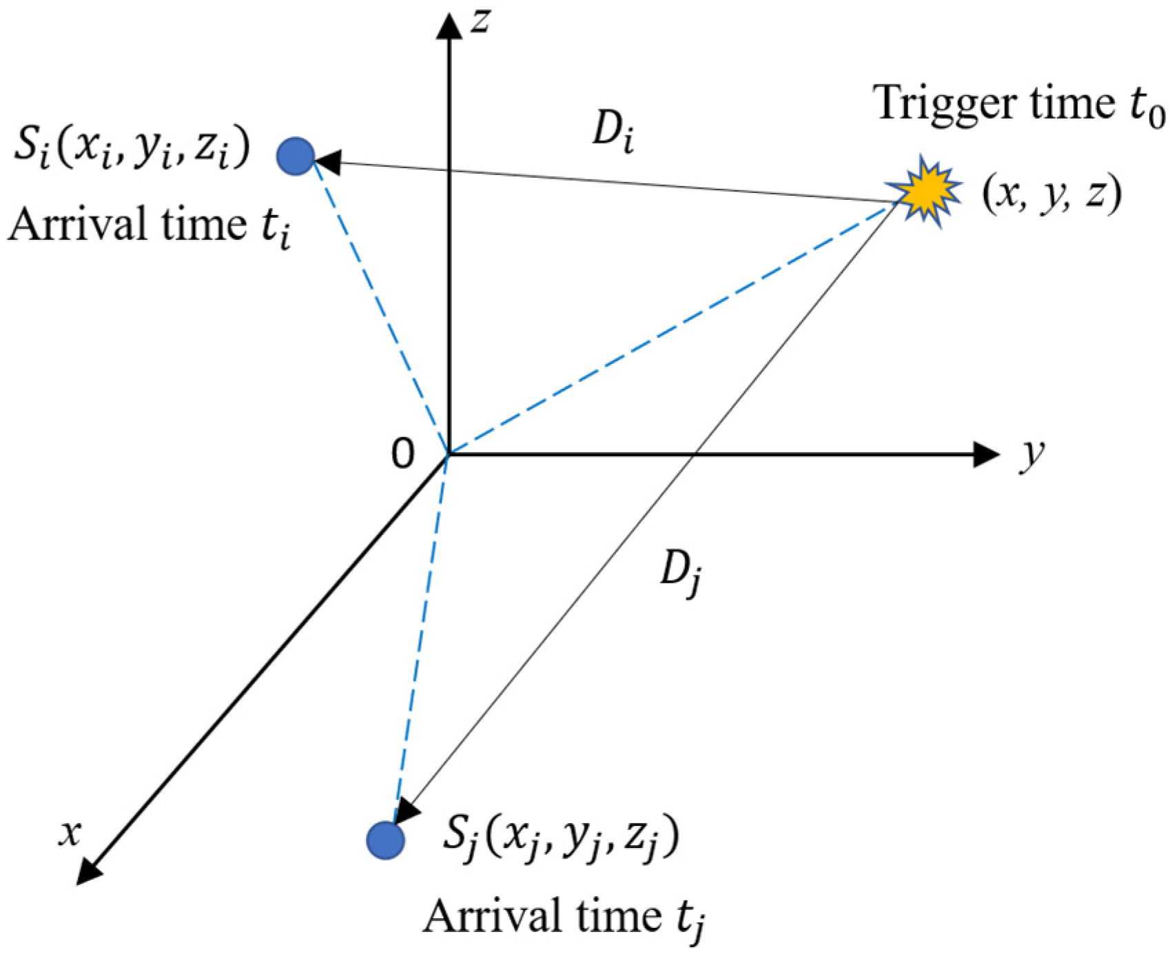
2. Methods
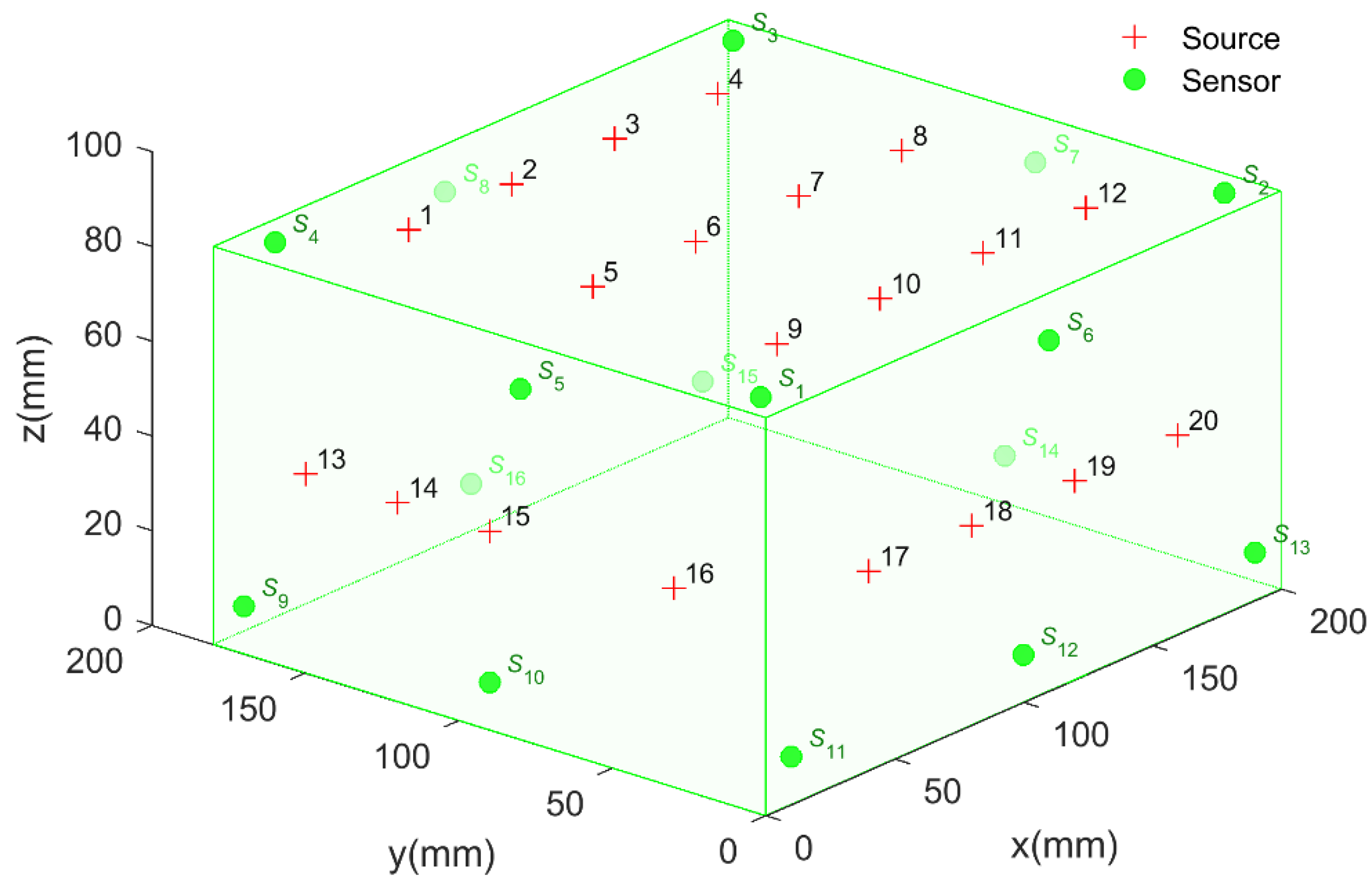
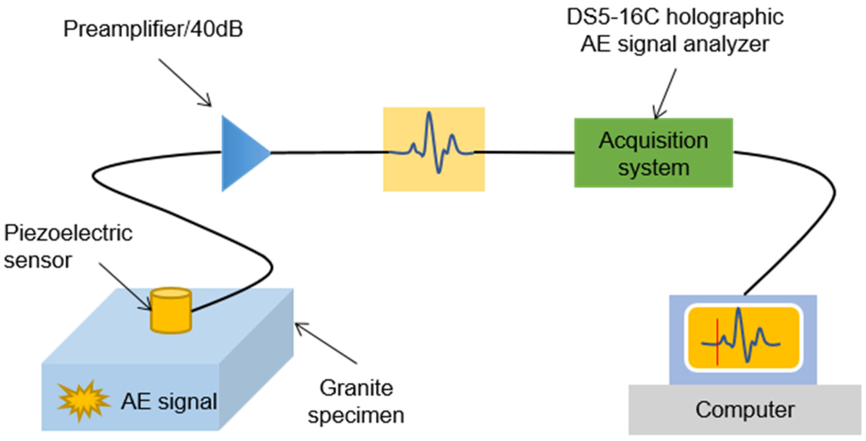
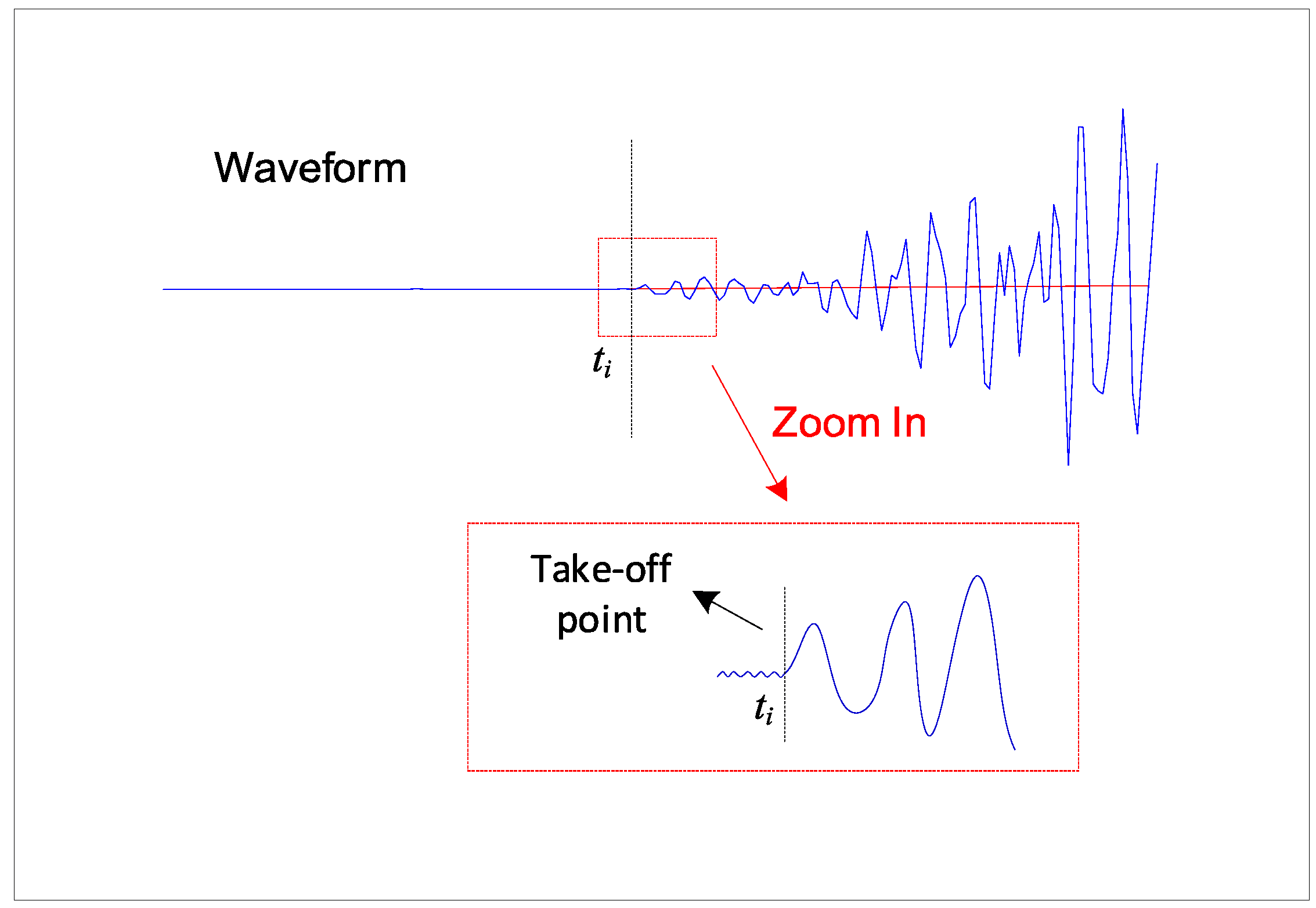
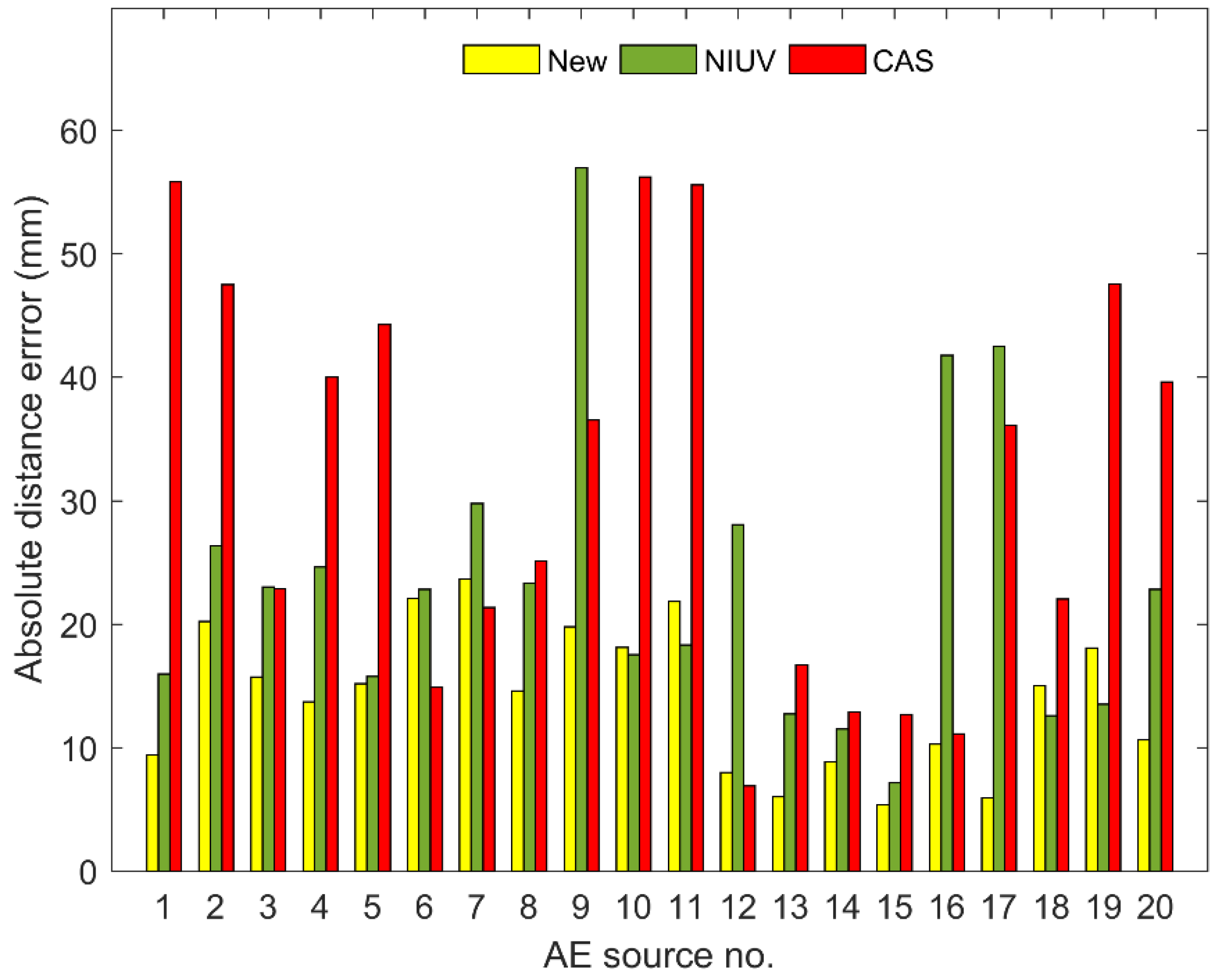
3. Experimental Verification by Pencil Lead Breaks
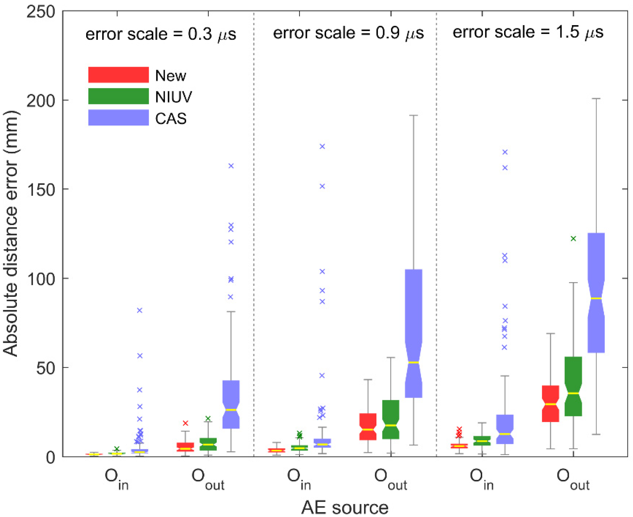
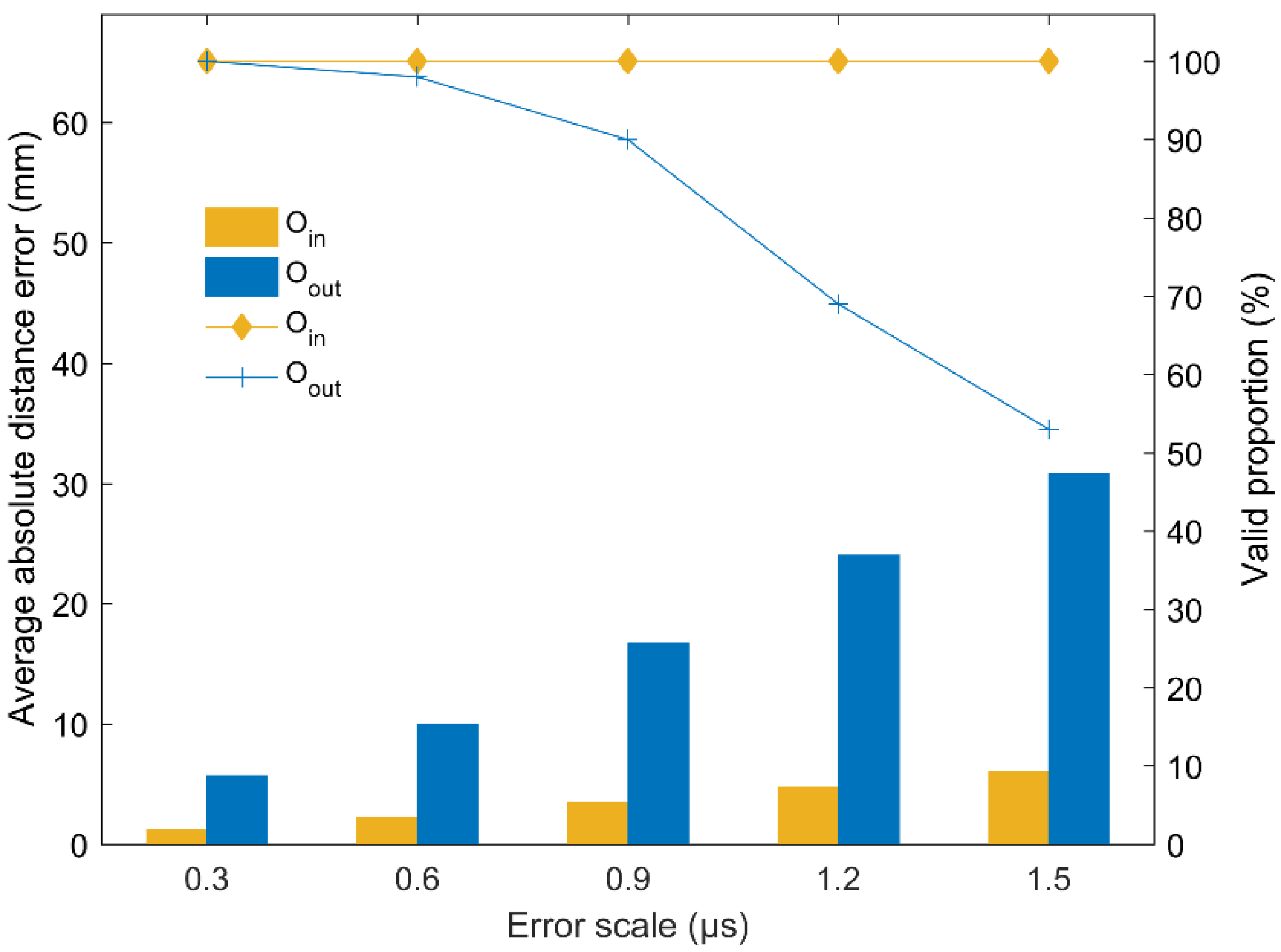
4. Simulation Analysis
5. Conclusions
Author Contributions
Funding
Conflicts of Interest
References
- Lu, C.; Dou, L.; Zhang, N.; Xue, J.; Wang, X.; Liu, H.; Zhang, J. Microseismic frequency-spectrum evolutionary rule of rockburst triggered by roof fall. Int. J. Rock Mech. Min. Sci. 2013, 64, 6–16. [Google Scholar] [CrossRef]
- Guo, Q.; Pan, J.; Cai, M.; Zhang, Y. Investigating the effect of rock bridge on the stability of locked section slopes by the direct shear test and acoustic emission technique. Sensors 2020, 20, 638. [Google Scholar] [CrossRef] [Green Version]
- Cai, X.; Zhou, Z.; Liu, K.; Du, X.; Zang, H. Water-weakening effects on the mechanical behavior of different rock types: Phenomena and mechanisms. Appl. Sci. 2019, 9, 4450. [Google Scholar] [CrossRef] [Green Version]
- Wang, Y.; Zhou, X.; Kou, M. Three-dimensional numerical study on the failure characteristics of intermittent fissures under compressive-shear loads. Acta Geotech. 2019, 14, 1161–1193. [Google Scholar] [CrossRef]
- Ma, D.; Wang, J.; Cai, X.; Ma, X.; Zhang, J.; Zhou, Z.; Tao, M. Effects of height/diameter ratio on failure and damage properties of granite under coupled bending and splitting deformation. Eng. Fract. Mech. 2019, 220, 4450. [Google Scholar] [CrossRef]
- Zhou, Z.; Wang, H.; Cai, X.; Chen, L.; Cheng, R. Damage Evolution and Failure Behavior of Post-Mainshock Damaged Rocks under Aftershock Effects. Energies 2019, 12, 4429. [Google Scholar] [CrossRef] [Green Version]
- Zhou, Z.; Cai, X.; Li, X.; Cao, W.; Du, X. Dynamic Response and Energy Evolution of Sandstone Under Coupled Static–Dynamic Compression: Insights from Experimental Study into Deep Rock Engineering Applications. Rock Mech. Rock Eng. 2019, 53, 1–27. [Google Scholar] [CrossRef]
- Muzet, A. Environmental noise, sleep and health. Sleep Med. Rev. 2007, 11, 135–142. [Google Scholar] [CrossRef]
- Zacarías, F.F.; Molina, R.H.; Ancela, J.L.C.; López, S.L.; Ojembarrena, A.A. Noise exposure in preterm infants treated with respiratory support using neonatal helmets. Acta Acust. United Acust. 2013, 99, 590–597. [Google Scholar] [CrossRef]
- Holford, K.M.; Eaton, M.J.; Hensman, J.J.; Pullin, R.; Evans, S.L.; Dervilis, N.; Worden, K. A new methodology for automating acoustic emission detection of metallic fatigue fractures in highly demanding aerospace environments: An overview. Prog. Aerosp. Sci. 2017, 90, 1–11. [Google Scholar] [CrossRef]
- Song, Z.; Konietzky, H.; Herbst, M. Bonded-particle model-based simulation of artificial rock subjected to cyclic loading. Acta Geotech. 2019, 14, 955–971. [Google Scholar] [CrossRef]
- Kou, M.; Lian, Y.; Wang, Y. Numerical investigations on crack propagation and crack branching in brittle solids under dynamic loading using bond-particle model. Eng. Fract. Mech. 2019, 212, 41–56. [Google Scholar] [CrossRef]
- Lu, C.; Liu, G.; Liu, Y.; Zhang, N.; Xue, J.; Zhang, L. Microseismic multi-parameter characteristics of rockburst hazard induced by hard roof fall and high stress concentration. Int. J. Rock Mech. Min. Sci. 2015, 76, 18–32. [Google Scholar] [CrossRef]
- Qi, L.; Zeng, Z.; Sun, L.; Rui, X.; Fan, F.; Yue, G.; Zhao, Y.; Feng, H. An Impact Location Algorithm for Spacecraft Stiffened Structure Based on Posterior Possibility Correlation. Sensors 2020, 20, 368. [Google Scholar] [CrossRef] [Green Version]
- Li, L.; Yang, K.; Bian, X.; Liu, Q.; Yang, Y.; Ma, F. A Gas Leakage Localization Method Based on a Virtual Ultrasonic Sensor Array. Sensors 2019, 19, 3152. [Google Scholar] [CrossRef] [Green Version]
- Fredianelli, L.; Nastasi, M.; Bernardini, M.; Fidecaro, F.; Licitra, G. Pass-by Characterization of Noise Emitted by Different Categories of Seagoing Ships in Ports. Sustainability 2020, 12, 1740. [Google Scholar] [CrossRef] [Green Version]
- Bolognese, M.; Fidecaro, F.; Palazzuoli, D.; Licitra, G. Port Noise and Complaints in the North Tyrrhenian Sea and Framework for Remediation. Environments 2020, 7, 17. [Google Scholar] [CrossRef] [Green Version]
- Ge, M. Analysis of source location algorithms Part I: Overview and non-iterative methods. J. Acoust. Emiss. 2003, 21, 14–28. [Google Scholar]
- Zhou, Z.; Rui, Y.; Zhou, J.; Dong, L.; Cai, X. Locating an Acoustic Emission Source in Multilayered Media Based on the Refraction Path Method. IEEE Access 2018, 6, 25090–25099. [Google Scholar] [CrossRef]
- Huang, W.; Zhang, W.; Li, F. Acoustic emission source location using a distributed feedback fiber laser rosette. Sensors 2013, 13, 14041–14054. [Google Scholar] [CrossRef] [Green Version]
- Zhang, Z.; Yang, G.; Hu, K. Prediction of Fatigue Crack Growth in Gas Turbine Engine Blades Using Acoustic Emission. Sensors 2018, 18, 1321. [Google Scholar] [CrossRef] [PubMed] [Green Version]
- Si, G.; Durucan, S.; Jamnikar, S.; Lazar, J.; Abraham, K.; Korre, A.; Shi, J.-Q.; Zavšek, S.; Mutke, G.; Lurka, A. Seismic monitoring and analysis of excessive gas emissions in heterogeneous coal seams. Int. J. Coal Geol. 2015, 149, 41–54. [Google Scholar] [CrossRef]
- Li, X.; Wang, Z.; Dong, L. Locating single-point sources from arrival times containing large picking errors (LPEs): The virtual field optimization method (VFOM). Sci. Rep. 2016, 6, 19205. [Google Scholar] [CrossRef] [PubMed] [Green Version]
- Li, Y.; Arce, G.R. A maximum likelihood approach to least absolute deviation regression. EURASIP J. Appl. Signal Process. 2004, 2004, 1762–1769. [Google Scholar] [CrossRef] [Green Version]
- Inglada, V. The calculation of the stove coordinates of a Nahbebens. Gerlands Beitrage Zur Geophys. 1928, 19, 73–98. [Google Scholar]
- Smith, J.O.; Abel, J.S. Closed-Form Least-Squares Source Location Estimation from Range-Difference Measurements. IEEE Trans. Acoust. 1987, 35, 1661–1669. [Google Scholar] [CrossRef]
- Zhou, Z.; Rui, Y.; Zhou, J.; Dong, L.; Chen, L.; Cai, X.; Cheng, R. A new closed-form solution for acoustic emission source location in the presence of outliers. Appl. Sci. 2018, 8, 949. [Google Scholar] [CrossRef] [Green Version]
- Li, Q.; Dong, L.; Li, X.; Yin, Z.; Liu, X. Effects of sonic speed on location accuracy of acoustic emission source in rocks. Trans. Nonferrous Met. Soc. China 2011, 21, 2719–2726. [Google Scholar] [CrossRef]
- Reuschlé, T.; Haore, S.G.; Darot, M. The effect of heating on the microstructural evolution of La Peyratte granite deduced from acoustic velocity measurements. Earth Planet. Sci. Lett. 2006, 243, 692–700. [Google Scholar] [CrossRef]
- Stanchits, S.; Vinciguerra, S.; Dresen, G. Ultrasonic velocities, acoustic emission characteristics and crack damage of basalt and granite. Pure Appl. Geophys. 2006, 163, 974–993. [Google Scholar] [CrossRef]
- Kundu, T. Acoustic source localization. Ultrasonics 2014, 54, 25–38. [Google Scholar] [CrossRef]
- Dong, L.; Zou, W.; Sun, D.; Tong, X.; Li, X.; Shu, W. Some Developments and New Insights for Microseismic/Acoustic Emission Source Localization. Shock Vib. 2019, 2019, 9732606. [Google Scholar] [CrossRef] [Green Version]
- Das, A.K.; Lai, T.T.; Chan, C.W.; Leung, C.K.Y. A new non-linear framework for localization of acoustic sources. Struct. Heal. Monit. 2019, 18, 590–601. [Google Scholar] [CrossRef]
- Dong, L.; Li, X. A Microseismic/Acoustic Emission Source Location Method Using Arrival Times of PS Waves for Unknown Velocity System. Int. J. Distrib. Sens. Netw. 2013, 9, 307489. [Google Scholar] [CrossRef]
- Dong, L.; Shu, W.; Han, G.; Li, X.; Wang, J. A Multi-Step Source Localization Method with Narrowing Velocity Interval of Cyber-Physical Systems in Buildings. IEEE Access 2017, 5, 20207–20219. [Google Scholar] [CrossRef]
- Geiger, L. Herdbestimmung bei erdbeben aus den ankunftszeiten. Nachrichten von der gesellschaft der wissenschaften zu Göttingen. Math. Klasse 1910, 4, 331–349. [Google Scholar]
- Geiger, L. Probability method for the determination of earthquake epicenters from the arrival time only. Bull. St. Louis Univ. 1912, 8, 60–71. [Google Scholar]
- Prugger, A.F.; Gendzwill, D.J. Microearthquake location: A nonlinear approach that makes use of a simplex stepping procedure. Bull. Seismol. Soc. Am. 1988, 78, 799–815. [Google Scholar]
- Rek, B.; Kvasnika, M. Differential Evolution Algorithm in the Earthquake Hypocenter Location. Pure Appl. Geophys. 2001, 158, 667–693. [Google Scholar] [CrossRef]
- Huang, Y.; Benesty, J.; Elko, G.W.; Mersereau, R.M. Real-time passive source localization: A practical linear-correction least-squares approach. IEEE Trans. Speech Audio Process. 2001, 9, 943–956. [Google Scholar] [CrossRef]
- Chan, Y.T.; Ho, K.C. A Simple and Efficient Estimator for Hyperbolic Location. IEEE Trans. Signal Process. 1994, 42, 1905–1915. [Google Scholar] [CrossRef] [Green Version]
- Kundu, T.; Nakatani, H.; Takeda, N. Acoustic source localization in anisotropic plates. Ultrasonics 2012, 52, 740–746. [Google Scholar] [CrossRef]
- Yin, S.; Cui, Z.; Kundu, T. Acoustic source localization in anisotropic plates with “Z” shaped sensor clusters. Ultrasonics 2018, 84, 34–37. [Google Scholar] [CrossRef]
- Dong, L.; Li, X.; Zhou, Z.; Chen, G.; Ma, J. Three-dimensional analytical solution of acoustic emission source location for cuboid monitoring network without pre-measured wave velocity. Trans. Nonferrous Met. Soc. China 2015, 25, 293–302. [Google Scholar] [CrossRef]
- Mahajan, A.; Walworth, M. 3-D position sensing using the differences in the time-of-flights from a wave source to various receivers. IEEE Trans. Robot. Autom. 2001, 17, 91–94. [Google Scholar] [CrossRef]
- Dong, L.; Shu, W.; Li, X.; Han, G.; Zou, W. Three Dimensional Comprehensive Analytical Solutions for Locating Sources of Sensor Networks in Unknown Velocity Mining System. IEEE Access 2017, 5, 11337–11351. [Google Scholar] [CrossRef]
- Li, X.; Dong, L. An efficient closed-form solution for acoustic emission source location in three-dimensional structures. AIP Adv. 2014, 4, 27110. [Google Scholar] [CrossRef]
- Zhou, Z.; Lan, R.; Rui, Y.; Zhou, J.; Dong, L.; Cheng, R.; Cai, X. A new acoustic emission source location method using tri-variate kernel density estimator. IEEE Access 2019, 7, 158379–158388. [Google Scholar] [CrossRef]
- Fang, W.; Liu, L.; Yang, J.; Shui, A. A non-iterative AE source localization algorithm with unknown velocity. J. Logist. Eng. Univ. 2016, 32, 1–7. [Google Scholar]
- Chen, J.C.; Yao, K.; Tung, T.L.; Reed, C.W.; Chen, D. Source localization and tracking of a wideband source using a randomly distributed beamforming sensor array. Int. J. High. Perform. Comput. Appl. 2002, 16, 259–272. [Google Scholar] [CrossRef]
- Friedlander, B. A Passive Localization Algorithm and Its Accuracy Analysis. IEEE J. Ocean. Eng. 1987, 12, 234–245. [Google Scholar] [CrossRef]
- Dong, L.; Li, X. Main Influencing Factors for the Accuracy of Microseismic Source Location. Sci. Technol. Rev. 2013, 31, 26–32. [Google Scholar]
- Li, N.; Wang, E.; Li, B.; Wang, X.; Chen, D. Research on the influence law and mechanisms of sensors network layouts for the source location. J. China Univ. Min. Technol. 2017, 46, 229–236. [Google Scholar]


| Sensor No. | x (mm) | y (mm) | z (mm) |
|---|---|---|---|
| 1 | 10 | 10 | 84 |
| 2 | 190 | 10 | 84 |
| 3 | 190 | 170 | 84 |
| 4 | 12 | 170 | 84 |
| 5 | 0 | 80 | 74 |
| 6 | 110 | 0 | 74 |
| 7 | 200 | 80 | 74 |
| 8 | 90 | 180 | 74 |
| 9 | 0 | 170 | 10 |
| 10 | 0 | 90 | 10 |
| 11 | 10 | 0 | 10 |
| 12 | 100 | 0 | 10 |
| 13 | 190 | 0 | 10 |
| 14 | 200 | 90 | 10 |
| 15 | 190 | 180 | 10 |
| 16 | 100 | 180 | 10 |
| AE Source No. | Methods | True Source Coordinates | AE Source No. | Methods | True Source Coordinates | ||||||
|---|---|---|---|---|---|---|---|---|---|---|---|
| x (mm) | y (mm) | z (mm) | Absolute Distance Error (mm) | x (mm) | y (mm) | z (mm) | Absolute Distance Error (mm) | ||||
| 1 | True position | 40.00 | 150.00 | 84.00 | - | 11 | True position | 120.00 | 30.00 | 84.00 | - |
| New | 39.41 | 155.99 | 91.20 | 9.39 | New | 122.41 | 27.06 | 105.49 | 21.83 | ||
| NIUV | 45.06 | 153.36 | 98.76 | 15.96 | NIUV | 121.12 | 28.89 | 102.25 | 18.32 | ||
| CAS | 22.93 | 184.95 | 124.06 | 55.84 | CAS | 124.99 | −7.32 | 124.90 | 55.60 | ||
| 2 | True position | 80.00 | 150.00 | 84.00 | - | 12 | True position | 160.00 | 30.00 | 84.00 | - |
| New | 81.71 | 157.52 | 102.72 | 20.25 | New | 165.02 | 26.15 | 88.87 | 7.98 | ||
| NIUV | 81.63 | 154.09 | 109.97 | 26.34 | NIUV | 168.22 | 19.31 | 108.64 | 28.09 | ||
| CAS | 75.08 | 176.28 | 123.30 | 47.53 | CAS | 162.45 | 27.51 | 89.94 | 6.90 | ||
| 3 | True position | 120.00 | 150.00 | 84.00 | - | 13 | True position | 0.00 | 150.00 | 42.00 | - |
| New | 116.21 | 139.77 | 95.29 | 15.70 | New | 4.38 | 153.93 | 43.16 | 6.00 | ||
| NIUV | 113.24 | 137.39 | 102.04 | 23.02 | NIUV | −3.45 | 161.10 | 47.16 | 12.72 | ||
| CAS | 109.53 | 137.50 | 100.06 | 22.89 | CAS | −1.24 | 166.26 | 45.55 | 16.69 | ||
| 4 | True position | 160.00 | 150.00 | 84.00 | - | 14 | True position | 0.00 | 120.00 | 42.00 | - |
| New | 162.47 | 155.20 | 96.46 | 13.72 | New | 8.07 | 119.25 | 45.63 | 8.88 | ||
| NIUV | 157.51 | 149.70 | 108.51 | 24.64 | NIUV | 5.99 | 120.77 | 51.78 | 11.49 | ||
| CAS | 170.47 | 167.40 | 118.50 | 40.03 | CAS | −5.73 | 122.43 | 53.30 | 12.90 | ||
| 5 | True position | 40.00 | 90.00 | 84.00 | - | 15 | True position | 0.00 | 90.00 | 42.00 | - |
| New | 47.66 | 91.18 | 97.05 | 15.18 | New | −5.03 | 89.00 | 43.61 | 5.37 | ||
| NIUV | 52.98 | 92.08 | 92.76 | 15.79 | NIUV | 3.59 | 88.76 | 48.05 | 7.14 | ||
| CAS | −1.69 | 75.60 | 87.68 | 44.27 | CAS | −1.31 | 87.30 | 54.35 | 12.71 | ||
| 6 | True position | 80.00 | 90.00 | 84.00 | - | 16 | True position | 0.00 | 30.00 | 42.00 | - |
| New | 82.90 | 92.47 | 105.77 | 22.10 | New | −2.96 | 20.74 | 45.29 | 10.26 | ||
| NIUV | 82.57 | 93.42 | 106.44 | 22.84 | NIUV | −29.37 | 0.31 | 43.72 | 41.80 | ||
| CAS | 91.28 | 98.21 | 89.18 | 14.88 | CAS | −2.17 | 19.16 | 41.00 | 11.10 | ||
| 7 | True position | 120.00 | 90.00 | 84.00 | - | 17 | True position | 40.00 | 0.00 | 42.00 | - |
| New | 120.37 | 92.86 | 107.47 | 23.65 | New | 40.78 | −4.08 | 46.24 | 5.94 | ||
| NIUV | 120.96 | 92.67 | 113.64 | 29.78 | NIUV | 64.39 | 33.30 | 52.26 | 42.53 | ||
| CAS | 120.35 | 93.10 | 105.14 | 21.37 | CAS | 19.41 | −29.33 | 46.59 | 36.12 | ||
| 8 | True position | 160.00 | 90.00 | 84.00 | - | 18 | True position | 80.00 | 0.00 | 42.00 | - |
| New | 159.08 | 89.84 | 98.57 | 14.60 | New | 81.59 | −14.73 | 44.64 | 15.04 | ||
| NIUV | 155.95 | 85.77 | 106.57 | 23.32 | NIUV | 85.10 | 8.22 | 50.02 | 12.57 | ||
| CAS | 149.81 | 72.34 | 98.68 | 25.13 | CAS | 89.04 | −19.24 | 47.82 | 22.04 | ||
| 9 | True position | 40.00 | 30.00 | 84.00 | - | 19 | True position | 120.00 | 0.00 | 42.00 | - |
| New | 32.69 | 18.83 | 98.59 | 19.78 | New | 117.06 | −17.83 | 41.36 | 18.08 | ||
| NIUV | 10.69 | −4.62 | 118.43 | 56.95 | NIUV | 110.03 | 8.16 | 37.85 | 13.54 | ||
| CAS | 26.84 | 13.36 | 113.73 | 36.52 | CAS | 111.05 | −30.89 | 6.96 | 47.56 | ||
| 10 | True position | 80.00 | 30.00 | 84.00 | - | 20 | True position | 160.00 | 0.00 | 42.00 | - |
| New | 79.71 | 29.91 | 102.10 | 18.10 | New | 156.77 | −9.53 | 45.37 | 10.61 | ||
| NIUV | 83.60 | 33.97 | 100.68 | 17.52 | NIUV | 156.78 | −21.83 | 47.76 | 22.80 | ||
| CAS | 76.27 | 8.47 | 135.82 | 56.24 | CAS | 167.59 | −38.22 | 34.72 | 39.64 | ||
| Sensor No. | x (mm) | y (mm) | z (mm) |
|---|---|---|---|
| 1 | 0 | 0 | 0 |
| 2 | 300 | 0 | 0 |
| 3 | 300 | 300 | 0 |
| 4 | 0 | 300 | 0 |
| 5 | 0 | 0 | 300 |
| 6 | 300 | 0 | 300 |
| 7 | 300 | 300 | 300 |
| 8 | 0 | 300 | 300 |
| 9 | 150 | 0 | 150 |
| 10 | 300 | 150 | 150 |
| 11 | 150 | 300 | 150 |
| 12 | 0 | 150 | 150 |
| 13 | 150 | 150 | 0 |
| 14 | 150 | 150 | 300 |
| 15 | 0 | 0 | 150 |
| 16 | 300 | 300 | 150 |
© 2020 by the authors. Licensee MDPI, Basel, Switzerland. This article is an open access article distributed under the terms and conditions of the Creative Commons Attribution (CC BY) license (http://creativecommons.org/licenses/by/4.0/).
Share and Cite
Zhou, Z.; Rui, Y.; Cai, X.; Cheng, R.; Du, X.; Lu, J. A Weighted Linear Least Squares Location Method of an Acoustic Emission Source without Measuring Wave Velocity. Sensors 2020, 20, 3191. https://doi.org/10.3390/s20113191
Zhou Z, Rui Y, Cai X, Cheng R, Du X, Lu J. A Weighted Linear Least Squares Location Method of an Acoustic Emission Source without Measuring Wave Velocity. Sensors. 2020; 20(11):3191. https://doi.org/10.3390/s20113191
Chicago/Turabian StyleZhou, Zilong, Yichao Rui, Xin Cai, Ruishan Cheng, Xueming Du, and Jianyou Lu. 2020. "A Weighted Linear Least Squares Location Method of an Acoustic Emission Source without Measuring Wave Velocity" Sensors 20, no. 11: 3191. https://doi.org/10.3390/s20113191