Abstract
We propose a distributed Kalman filter for a sensor network under model uncertainty. The distributed scheme is characterized by two communication stages in each time step: in the first stage, the local units exchange their observations and then they can compute their local estimate; in the final stage, the local units exchange their local estimate and compute the final estimate using a diffusion scheme. Each local estimate is computed in order to be optimal according to the least favorable model belonging to a prescribed local ambiguity set. The latter is a ball, in the Kullback–Liebler topology, about the corresponding nominal local model. We propose a strategy to compute the radius, called local tolerance, for each local ambiguity set in the sensor network, rather than keep it constant across the network. Finally, some numerical examples show the effectiveness of the proposed scheme.
1. Introduction
Modern problems involve a large number of sensors forming a sensor network and taking measurements from which we would like to infer quantities not accessible to observation possibly at each node location. These problems can be classified as filtering problems whose solution is given by the Kalman filter. On the other hand, its implementation is very expensive in terms of data transmission; indeed, we require that all sensors can exchange their measurements. Such a limitation disappears by considering distributed filtering [1,2,3,4,5,6,7,8,9]. The key idea is that the communication among the nodes is limited.
In the simplest distributed strategy, the state estimate of a node (i.e., local unit) is computed by using only the observations from its neighbors. Such a strategy, however, appears to be not very effective. A remarkable progress has been reached by distributed Kalman filtering with consensus [10,11,12,13] and diffusion strategies [14,15]. These distributed approaches are characterized by several communication stages during each time step. For instance, in the first stage, the local units exchange their observations and then they can compute their local estimate; in the final stage, the local units exchange their local estimate and compute the final estimate using a consensus or a diffusion scheme. Many important challenges have been addressed in distributed filtering. For instance, the issues about limited observability, network topologies that restrict allowable communications, and communication noises between sensors are considered in [16]; the case in which the sensor network is subject to transmission delays is considered in [17]; and the cases of missing measurements and absence of communication among the nodes are analyzed in [18,19], respectively. It is worth observing that distributed state estimation can be performed also through different principles [20,21,22,23,24,25]. For instance, each node can transmit its measurements to a fusion center and then the latter computes the state estimate.
An important aspect in filtering applications is that the nominal model does not correspond to the actual one. Risk sensitive Kalman filtering [26,27,28] addresses this problem by penalizing large errors. The severity of this penalization is tuned by the so-called risk sensitivity parameter: the larger the risk sensitivity parameter is, the more large errors are penalized. A refinement of these filters is given by robust Kalman filtering where the uncertainty is expressed incrementally [29,30,31,32]. More precisely, for each time step, the state estimator minimizes the prediction error according to the least favorable model belonging to a prescribed ambiguity set. The latter is a ball in the Kullback–Leibler (KL) topology whose center is the nominal model. The radius of this ball is called tolerance and it represents the discrepancy budget between the actual and the nominal model allowed for the corresponding time step. It is worth noting that the ambiguity set can be formed also by using different types of divergence (see, for instance, [33,34,35]).
The problem of distributed Kalman filtering under model uncertainty has been considered as well (see, e.g., [36,37,38]). In the present paper, we consider the distributed robust Kalman filter with diffusion step proposed in [39]. Here, the local estimate of each node is computed by using the robust Kalman filter in [29]. In this scenario, the least favorable model is the one used to compute the robust Kalman filter of the global model. Accordingly, we have one ambiguity set corresponding to the global model, which contains the actual model, and the local ambiguity sets corresponding to the nodes of the network. The centers of those balls are known because they are given by the nominal model. The local tolerances corresponding to the local ambiguity sets of the nodes are set equal to the one of the global ambiguity set. On the other hand, the local ambiguity set of a node corresponds to a local model which is just a part of the global model. Accordingly, taking all the local tolerances uniform across the network and equal to the global one may not be the best choice.
The main contribution of this paper is to propose a robust distributed Kalman filter as in [39] where the local tolerance for each node is customized. In this way, the local tolerance is non-uniform and time-varying across the network. We show through some simulation studies that the performance of the predictions is improved. Moreover, we show that, if the tolerance corresponding to the global ambiguity set is sufficiently small, then the local tolerances across the network are constant in the steady-state condition. Accordingly, it is also possible to simplify the distributed scheme by replacing the time-varying tolerances with the steady-state values.
The organization of this paper is as follows. In Section 2, we provide the background about robust Kalman filtering whose uncertainty is expressed incrementally. In Section 3, the distributed robust Kalman filter with local uniform tolerance is reviewed. In Section 4, we introduce the distributed robust Kalman filter with non-uniform local tolerance. In Section 5, we perform some numerical experiments to check the performance of the proposed distributed scheme. In Section 6, we propose an efficient approximation of the distributed robust Kalman filter with non-uniform local tolerance. Finally, in Section 7, we draw the conclusions.
Notation: denotes the matrix having entry in position ; is the transposition of matrix A; and means that matrix A is positive (semi)-definite. denotes a block-diagonal matrix whose blocks in the main block diagonal are . Given a squared matrix A, and denote the trace and the determinant of A, respectively. Given two matrices A and B, denotes their Kronecker product. means that x is a Gaussian random vector with mean m and covariance matrix K.
2. Background
In this section, we review the robust Kalman filter proposed in [29], which represents the “building block” used throughout the paper. Consider the nominal state-space model
where , , , , is the state process, is the observation process, is normalized white Gaussian noise (WGN), and is a deterministic signal. It is assumed that is independent from the initial state . We also assume that the noise entering in the state process and the one entering in the observation process are independent, i.e., we assume that . Finally, the state-space model in Equation (1) is considered to be reachable and observable. Let denote the nominal transition probability density of given . Notice that is Gaussian by construction and it is straightforwardly given by Equation (1).
We assume that the (unknown) actual transition probability belongs to the ambiguity set which is a closed ball centered in in the KL topology:
with
, and is defined as the actual conditional probability density of given . The mismatch modeling budget allowed for each time step is represented by the parameter , which is called tolerance. The robust estimator of given for the nominal model in Equation (1) is given by solving the following minimax problem:
where is the set of all estimators whose variance is finite under any model in the ambiguity set ,
is the estimation error under the transition density . In [29], it is proved that the estimator solution to the problem in Equation (3) has the following Kalman-like structure:
where
Parameter is called risk sensitivity parameter. It is worth noting that, given and , the equation always admits a unique solution in and such that: , . In the special case that , i.e., the nominal model coincides with the actual model, then and thus Equation (4) degenerates in the usual Kalman filter.
Remark 1.
It is worth noting that the robust Kalman filter is well defined also in the case that the ambiguity set Equation (2) is defined by a time-varying tolerance, i.e., instead of c. However, we prefer to keep c constant in Equation (3) because in the following we assume that the actual (global) model is the solution to Equation (3) with constant tolerance c, in order to simplify the setup.
3. Distributed Robust Kalman Filtering with Uniform Local Tolerance
In this section, we review the distributed robust Kalman filter presented in [39]. Consider a network made by N sensors. The latter are connected if they can communicate with each other. Accordingly, every sensor k has a set of neighbors which is denoted by . In particular, that is each node is connected with itself. The number of neighbors of node k is denoted by . The corresponding adjacency matrix is defined as
We assume that every node collects a measurement at time t and the corresponding nominal state-space model is
where and , with , are independent normalized WGNs. It is worth noting that the actual state-space model for each node is unknown. By stacking Equation (5) for every k, it is possible to rewrite such sensor network as Equation (1) where:
Accordingly, Equation (4) represents the centralized robust Kalman filter. Defining , with , and
the Kalman gain for Equation (5) becomes, using the matrix inversion lemma,
Since the nominal model in Equation (5) does not coincide with the actual one and each node k can only exploit information shared by its neighbors , the aim of distributed robust Kalman filtering is to compute a prediction of the state for every node k by using only the local information, taking into account the model uncertainty. In the case that the node k has access to all measurements across all the nodes in the network, then coincides with Equation (4) which can be written, using the parameterization in Equations (6) and (7) as
where , , , and . In the case that not all the measurements in the network are accessible to node k, then the target is to compute a state prediction of which is as similar as possible to the global state prediction.
Assume that the node k can collect the measurements from its neighbors . Then, the corresponding local nominal state-space model is
The latter can be rewritten in the compact form
where is the input noise and is the output; and are given by stacking and , with , respectively. Moreover, is given by stacking with , and is a block diagonal matrix whose main blocks are with . In addition, defining and it results that
We conclude that the one-step ahead predictor of at node k is similar to the one in Equation (8) but now we need to discard the terms for which . It is worth noting that the latter represents an intermediate local prediction of at node k, and it is denoted as . Allowing that the connected nodes can exchange their intermediate estimates, then each node can update the prediction at node k in terms of both and with . More precisely, consider a matrix such that
Therefore, the final predicted state at node k is given by means of the so-called diffusion step [14]:
To sum up, in the diffusion scheme, each local unit uses the measurements and the intermediate local predictions from its neighbors. The resulting scheme is explained through Algorithm 1.
| Algorithm 1 Distributed robust Kalman filter with uniform local tolerance at time t. |
|
It is worth noting that is computed by using the robust Kalman scheme in Equation (4) applied to the local model in Equation (10). In addition, c is the same for any node that is c takes a uniform value over the sensor network. In particular, the tolerance c is the same for both the centralized and the distributed Kalman filter. This strategy for the selection of the tolerance does not ensure that the least favorable model computed at node k is compatible with the one of the centralized filter. However, in the case of large deviations of the least favorable model corresponding to the centralized problem, it is very likely that the predictor at node k using Algorithm 1 is better than the one which assumes that the nominal and actual models coincide. Finally, in the case that , i.e., the nominal model coincides with the actual one, Algorithm 1 boils down to the distributed Kalman filter with diffusion step in [14].
4. Distributed Robust Kalman Filtering with Non-Uniform Local Tolerance
We investigate the possibility to assign a possibly different local tolerance to each node that is the local tolerance is not uniform across the sensor network. Recall that the least favorable model is given by the minimax problem in Equation (3), with constant tolerance c, and the corresponding optimal estimator is given by the centralized robust Kalman filter in Equation (4).
Consider the centralized problem in Equation (3). Let
denote the pseudo-nominal and the least favorable conditional probability densities of given the past observations , respectively. Recall that is the nominal transition density of the state space model in Equation (1) and thus
In [29], it has been shown that the optimal solution to Equation (3) is Gaussian. Accordingly, in view of Equation (15), the corresponding least favorable density of given is Gaussian:
It is clear then that the minimax problem in Equation (3) can be written by replacing and with and , respectively. Then, the equivalent minimax problem is
where the ambiguity set is a ball about the pseudo-nominal density
formed by the KL divergence between and :
Since and are Gaussian distributed, we have
It is well known that also represents the negative log-likelihood of the model under the actual model , [40,41,42]. Accordingly, c represents an upper bound of the negative log-likelihood and it can be found as follows. Fix the nominal state space model and collect the data where , , . Let be the negative log-likelihood of this nominal model using the collected data. Then, fix . Clearly, we need to assume that the state is accessible to observation (or its estimate is reasonably good) to compute c.
Theorem 1
(Levy & Nikoukhah [30]). Let be the nominal density with mean and covariance matrix partitioned as
according to the dimension of and , respectively. The least favorable density solution to Equation (18) has mean and covariance matrix as follows:
Let
denote the nominal and least favorable error covariance matrices of given . Then,
and is the unique value for which
The above result provides a way to compute . Indeed, once the centralized robust Kalman filter in Equation (4) has been computed, the mean and the covariance matrix of are given, in view of Equation (17), by
where
From and , we can compute the nominal and least favorable density for each node. Consider the state-space model in Equation (10) for node k. Let . Then, the nominal transition probability at node k, in view of Equation (10), is
Then,
denotes the pseudo-nominal conditional probability density of given the past observations at node k. Since , and in view of Equation (23), we have
where
and
Such a result is not surprising, indeed is given by marginalizing with respect to with . Roughly speaking, this means that , and are obtained from , and as follows:
- is the vector obtained from by deleting the elements from to for any .
- is the matrix obtained from by deleting the columns from to for any .
- is the matrix obtained from by deleting the rows and the columns from to for any .
Accordingly, we can compute the least favorable density at node k, say , by marginalizing with respect to with . Therefore, we have
with
where in the last equality we exploit Equation (22). It remains to design the robust filter to compute the intermediate prediction .
Remark 2.
At this point, it is worth doing a digression about Algorithm 1. The intermediate prediction at node k is the solution to the following minimax problem
where
and is the set of all estimators whose variance is finite under any model in the ambiguity set . Moreover, in view of Theorem 1, the least favorable density solution to Equation (26) is such that . It is worth noting that the best estimator at node k would be the one constructed from . On the other hand, the problem in Equation (26) implies neither nor .
Clearly, one would design the intermediate estimator at node k by using . However, the latter is not available at node k, and it is only known by a “central unit”, i.e., a unit knowing the global model, but neither collecting measurements nor computing predictions. Moreover, the transmission of the mean and the covariance matrix of would be more expensive in terms of transmission costs. As alternative, we can consider a minimax problem whose least favorable model is such that :
where
and coincides with the number of rows of . Under the above scheme, the central unit only transmits the local tolerance to each node in the network. The procedure which implements this optimized strategy of distributed robust Kalman filtering is outlined in Algorithm 2.
| Algorithm 2 Distributed robust Kalman filter with non-uniform local tolerance at time t. |
|
Least Favorable Performance
We show how to evaluate the performance of the previously introduced distributed algorithm with non-uniform local tolerance and diffusion step with respect to the least favorable model solution of the centralized problem in Equation (3). More precisely, we show how to compute the mean and the variance of the prediction error for each node k in the network. In [29,34], it is shown that the least favorable model can be characterized through a state-space model over a finite interval as follows. Let , where is the least favorable state process. Then, the least favorable model takes the form
where is normalized WGN, independent from , and . Moreover,
where is such that ,
The matrix is computed from the backward recursion
where the final point is initialized with .
Let denote the least favorable state prediction error of node k at time t using Algorithm 2 or Algorithm 1. Define the vector containing all the errors across the network
Using the same reasonings in [39], it is not difficult to prove that obeys the following dynamics
where
, , and are such that and . Finally, denotes the vector of ones. Then, we combine Equation (35) with the model for in Equation (34):
where ,
Taking the expectation of Equation (36), we obtain
In view of the fact that has mean equal to and for , it is not difficult to see that . This implies that is a zero mean stochastic process or, equivalently, all the predictors are unbiased. Next, we show how to derive the variance of the prediction errors. Let . In view of the fact that is normalized WGN, by Equation (36), we have that is given by solving the following Lyapunov equation
We partition as follows:
where , and . Notice that contains in the main block diagonal the covariance matrices of the estimation error at each node. Accordingly, the least favorable mean square deviation is given by
where is the variance of the prediction error at node k. Finally, we have the following convergence result for the proposed distributed algorithm.
Proposition 1.
Let be a reachable pair and be an observable pair for any k. Let W be an arbitrary diffusion matrix satisfying Equation (11). Then, there exists sufficiently small such that, for any arbitrary initial condition and , the sequence , , generated by Equation (39) converges to over as . Moreover, we have , , and . In particular, corresponds to the unique solution of the algebraic Lyapunov equation
with Schur stable. Accordingly, converges over as .
Proof.
First, notice that the observability condition on the pairs implies the observability of . Since the global model is reachable and observable, the robust centralized Kalman filter converges provided that c is sufficiently small (see [43,44]). As a consequence, as . Accordingly, in view of Equation (17), and, thus, in view of Equation (22), . Since and are submatrices of and , respectively, we have that and . Accordingly, in view of Equation (30), we have that where
In [30], it has been shown that as , and thus . Since and are submatrices of and , respectively, we have that . Accordingly, in view of Equation (30), we have that as .
In view of ([43], Proposition 5.3), we conclude that the robust local Kalman filter at node k converges because: the local state-space model is reachable and observable; is sufficiently small provided that c is sufficiently small as well.
Finally, the remaining part of the proof follows the one in ([39], Section IV-A) (see also [45]). □
It is worth noting that Proposition 1 guarantees that is bounded because is Schur stable. This means that the prediction errors over the network have finite variance, i.e., the Kalman gains of the local filters are stabilizing. The proof above also shows that, in the case , i.e., the nominal model coincides with the actual one, Algorithm 2 boils down to the distributed Kalman filter with diffusion step proposed in [14].
5. Numerical Examples
In this section, we test the performance of the distributed Kalman filters with uniform versus non-uniform local tolerance. More precisely, we consider the problem in [39] to track the position of a projectile from position observations corrupted by noise and coming from a network of sensors. The latter is shown in Figure 1.
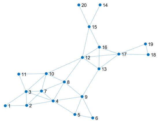
Figure 1.
Network of 20 sensors for measuring the noisy positions of the projectile.
The model for the projectile motion is
where
, with , and , with v denoting the velocity and p the position in the three spatial components. We discretize Equation (43) by using a sampling time equal to . In this way, the model becomes
where is the sampled version of , and . Assuming that every sensor can measure only along two spatial components, the output matrix of the kth node can be of the type
Every output matrix is assigned randomly to each node, with the constraint that the local state-space model in Equation (10) associated to each node must be observable for every node to guarantee the convergence of the robust Kalman filters at every node. Thus, if any node violates the constraint, all the output matrices are discarded and reassigned. Then, we choose , , where and P is a permutation matrix which is randomly generated for any node. The initial state is Gaussian distributed and whose covariance matrix is .
In the numerical simulations, the following Kalman filters are considered: the centralized Kalman filter (KFC); the centralized robust Kalman filter (RKFC); the distributed Kalman filter with diffusion step (KFD) proposed in [14]; the distributed robust Kalman with diffusion step and uniform local tolerance (RKFDU) proposed in [39] and reviewed in Section 3; and the distributed robust Kalman filter with diffusion step and non-uniform local tolerance (RKFDNU) proposed in Section 4. For the distributed filters, the diffusion matrix W is defined as
where represents the total number of neighbors of node l while is chosen such that Equation (11) holds.
5.1. First Example
We assume that the actual model is contained in the ambiguity set Equation (2) with . Figure 2 shows the least favorable mean squared deviation across the network. We notice that converges at the steady-state for all the distributed versions of the Kalman filter. RKFDNU performs slightly better that RKFDU and both perform consistently better than KFD. Finally, all of them perform worse than the centralized versions, and RKFC results the best.
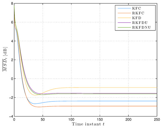
Figure 2.
Least favorable mean square deviation across the network with tolerance .
However, the situation is more salient if we consider the steady-state least favorable for each node (see Figure 3a): RKFDNU performs slightly better than RKFDU for the majority of the nodes. However, there is a clear difference for nodes 18 and 19 which are more susceptible to model uncertainty: RKFDNU performs better than RKFDU.
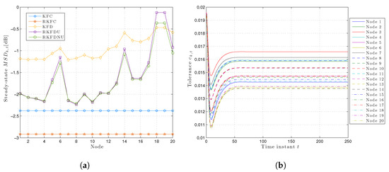
Figure 3.
(a) Least favorable mean square deviation for each node in the steady-state with tolerance . (b) Time-variant local tolerances for each node over time with .
Figure 3b shows the behavior of the local tolerances over the time for RKFDNU. As expected, every converges to a constant value. However, the latter is different from the tolerance c of the centralized minimax problem.
Finally, Figure 4a,b shows the risk sensitivity parameters at every node for RKFDU and RKFDNU. We can observe that the risk sensitivity parameters of RKFDU takes larger values than the ones of RKFDNU. Accordingly, the inferior performance of RKFDU is due by the fact that the robust local filters are too conservative.
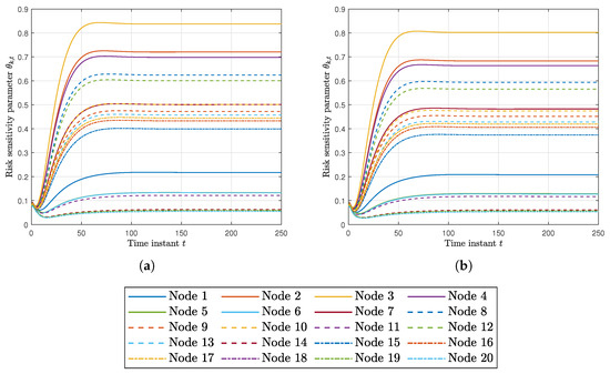
Figure 4.
(a) Risk sensitivity parameter for each node using RKFDU with tolerance . (b) Risk sensitivity parameter for each node using RKFDNU with tolerance .
5.2. Second Example
In the second experiment, we consider a larger deviation between the actual model and the nominal one, i.e., we choose .
Figure 5 and Figure 6a show the least favorable mean square deviation across the network and for each node in the steady-state. The situation is similar to the previous one, but the difference among RKFD, RKFDU, and RKFDNU is more evident. In particular, the steady-state value of for using RKFDNU is clearly better than the ones corresponding to KFD and RKFDU.
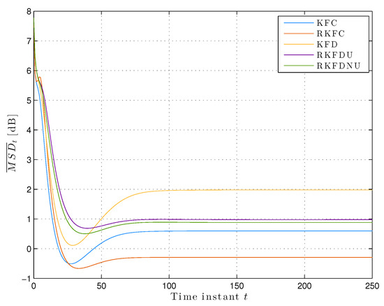
Figure 5.
Least favorable mean square deviation across the network with tolerance .
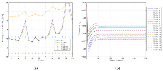
Figure 6.
(a) Least favorable mean square deviation for each node in the steady-state with tolerance . (b) Time-variant local tolerances for each node over time with .
In addition, Figure 6b shows the tolerances at every node over the time. As expected, the latter are higher than the ones with . Indeed, the uncertainty now is greater than before and thus the robust local filters now must be more conservative than before.
Finally, we study how the least favorable MSD for each node correlates with the topology of the sensor network. Figure 7a,b shows two additional sensor networks obtained from the original network of Figure 1 by adding connections only to some nodes. More precisely, the density of the original network, i.e., number of connections over all possible connections, is ; the density of the networks in Figure 7a,b is and , respectively.
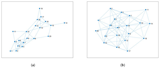
Figure 7.
(a) Sensor network with density . (b) Sensor network with density .
Figure 8a,b shows the results obtained by RKFDNU with the three different sensor networks. As expected, the increase of the degrees of the nodes, and consequently of the connections in the network, reduces the least favorable MSD related to those nodes at steady-state and the total least favorable MSD across the network. In conclusion, by adding edges the performance of RKFDNU tends to the one obtained in the centralized case (RKFC), where the nodes are considered all connected to each other.
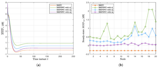
Figure 8.
Performance of RKFDNU across the three networks compared with RKFC. (a) Least favorable mean square deviation with tolerance . (b) Least favorable mean square deviation for each node in the steady-state with tolerance .
6. Efficient Algorithm
Proposition 1 suggests a simplified version of Algorithm 2. Indeed, if c is sufficiently small, then converges to in the steady state for every node of the network. Accordingly, the central unit can compute and transmit it to any node once. In this way, the transmission costs are reduced. The resulting procedure is outlined in Algorithm 3.
| Algorithm 3 Efficient distributed robust Kalman filter with non-uniform local tolerance at time t. |
|
We compared this algorithm, hereafter called RKFDNU2, with RKFDNU: the performance in practice is the same. Figure 9 shows their least favorable mean square deviation across the network in the scenario of Section 5.2 in the first 50 time steps. Finally, Figure 10a,b shows the risk sensitivity parameters for RKDFNU and RKFDNU2, respectively: there is a slight difference. However, we saw that such a difference disappears after 20 time steps. We conclude that the efficient scheme RKFDNU2 represents a good approximation of RKFDNU.
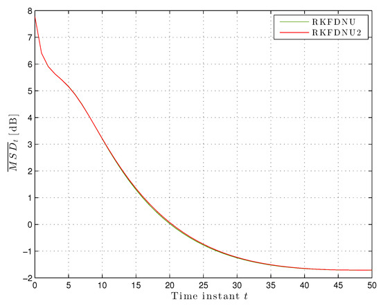
Figure 9.
Least favorable mean square deviation across the network with tolerance .
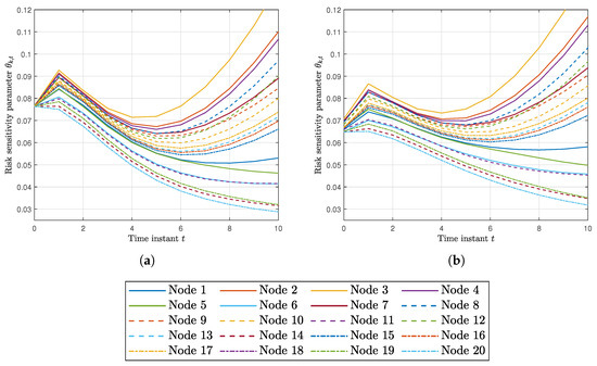
Figure 10.
(a) Risk sensitivity parameter for each node using RKFDNU with tolerance . (b) Risk sensitivity parameter for each node using RKFDNU2 with tolerance .
Finally, Table 1 summarizes the performance of RKFC, RKFDU, RKFDNU, and RKFDNU2 obtained with tolerance . The considered values are the least favorable MSD across the network at steady-state, the average among every node of the tolerances at steady-state, the average among every node of the risk sensitivity parameter at steady-state, and the occurred communications between the central unit and the local nodes in the whole time span. In particular, concerning the communication:

Table 1.
Summary of the performance of the different algorithms with tolerance .
- in RKFDU, the central unit transmits the uniform tolerance to each node at once (at the beginning);
- in RKFDNU, the central unit transmits the local tolerances to each node at every time step;
- in RKFDNU2, the central unit transmits the steady-state local tolerances to each node at once (at the beginning).
7. Conclusions
In this article, the problem of distributed robust Kalman filtering for a sensor network is considered. More precisely, we consider a distributed scheme with diffusion step and the intermediate estimate is designed in order to be optimal according to the least favorable model belonging to a prescribed local ambiguity set. The latter is a ball about the local nominal model and the radius of this ball is the local tolerance. In this paper, we propose an algorithm in which the local tolerance of each node is different and suitably computed by the central unit. We also consider a more efficient implementation of the algorithm where the central unit computes and transmits the steady-state local tolerances for every node at once. In this way, the communication between the central unit and the local nodes is reduced. Through some numerical examples, we showed that the proposed algorithm performs better than the one with a uniform local tolerance across the network.
Author Contributions
Conceptualization, A.E., F.G., G.G. and M.Z.; methodology, A.E., F.G., G.G. and M.Z.; simulations, A.E., F.G., G.G. and M.Z.; supervision, M.Z.; All the authors contributed equally. All authors have read and agreed to the published version of the manuscript.
Funding
Part of this work has been supported by the MIUR (Italian Minister for Education) under the initiative “Departments of Excellence” (Law 232/2016).
Conflicts of Interest
The authors declare no conflict of interest.
References
- Wu, H.N.; Wang, H.D. Distributed consensus observers-based H∞ control of dissipative PDE systems using sensor networks. IEEE Trans. Control Netw. Syst. 2015, 2, 112–121. [Google Scholar] [CrossRef]
- Orihuela, L.; Millán, P.; Vivas, C.; Rubio, F.R. Distributed control and estimation scheme with applications to process control. IEEE Trans. Control Syst. Technol. 2015, 23, 1563–1570. [Google Scholar] [CrossRef]
- Sadamoto, T.; Ishizaki, T.; Imura, J. Average state observers for large-scale network systems. IEEE Trans. Control Netw. Syst. 2017, 4, 761–769. [Google Scholar] [CrossRef]
- Wang, S.; Ren, W.; Chen, J. Fully distributed dynamic state estimation with uncertain process models. IEEE Trans. Control Netw. Syst. 2017, 5, 1841–1851. [Google Scholar] [CrossRef]
- Dormann, K.; Noack, B.; Hanebeck, U. Optimally distributed Kalman filtering with data-driven communication. Sensors 2018, 18, 1034. [Google Scholar] [CrossRef] [PubMed]
- Ruan, Y.; Luo, Y.; Zhu, Y. Globally optimal distributed Kalman filtering for multisensor systems with unknown inputs. Sensors 2018, 18, 2976. [Google Scholar] [CrossRef]
- Gao, S.; Chen, P.; Huang, D.; Niu, Q. Stability analysis of multi-sensor Kalman filtering over lossy networks. Sensors 2016, 16, 566. [Google Scholar] [CrossRef]
- Kordestani, M.; Samadi, M.; Saif, M. A distributed fault detection and isolation method for multifunctional spoiler system. In Proceedings of the 2018 IEEE 61st International Midwest Symposium on Circuits and Systems, Windsor, ON, Canada, 5–8 August 2018; pp. 380–383. [Google Scholar]
- Scott, S.; Blocker, A.; Bonassi, F.; Chipman, H.; George, E.; McCulloch, R. Bayes and big data: The consensus Monte Carlo algorithm. EFaBBayes 250th Conf. 2013, 16. [Google Scholar] [CrossRef]
- Spanos, D.P.; Olfati-Saber, R.; Murray, R.M. Approximate distributed Kalman filtering in sensor networks with quantifiable performance. In Proceedings of the Fourth International Symposium on Information Processing in Sensor Networks, Boise, ID, USA, 15 April 2005; pp. 133–139. [Google Scholar]
- Olfati-Saber, R. Distributed Kalman filter with embedded consensus filters. In Proceedings of the 44th IEEE Conference on Decision and Control, Seville, Spain, 15 December 2005; pp. 8179–8184. [Google Scholar]
- Olfati-Saber, R. Distributed Kalman filtering for sensor networks. In Proceedings of the 2007 46th IEEE Conference on Decision and Control, New Orleans, LA, USA, 12–14 December 2007; pp. 5492–5498. [Google Scholar]
- Carli, R.; Chiuso, A.; Schenato, L.; Zampieri, S. Distributed Kalman filtering based on consensus strategies. IEEE J. Sel. Areas Commun. 2008, 26, 622–633. [Google Scholar] [CrossRef]
- Cattivelli, F.S.; Sayed, A.H. Diffusion strategies for distributed Kalman filtering and smoothing. IEEE Trans. Autom. Control 2010, 55, 2069–2084. [Google Scholar] [CrossRef]
- Yang, S.; Huang, T.; Guan, J.; Xiong, Y.; Wang, M. Diffusion Strategies for Distributed Kalman Filter with Dynamic Topologies in Virtualized Sensor Networks. Mob. Inf. Syst. 2016, 2016, 8695102. [Google Scholar] [CrossRef]
- Ji, H.; Lewis, F.L.; Hou, Z.; Mikulski, D. Distributed information weighted Kalman consensus filter for sensor networks. Automatica 2017, 77, 18–30. [Google Scholar] [CrossRef]
- Yang, H.; Li, H.; Xia, Y.; Li, L. Distributed Kalman filtering over sensor networks with transmission delays. IEEE Trans. Cybern. 2020, 1–11. [Google Scholar] [CrossRef] [PubMed]
- Kordestani, M.; Dehghani, M.; Moshiri, B.; Saif, M. A new fusion estimation method for multi-rate multi-sensor systems with missing measurements. IEEE Access 2020, 8, 47522–47532. [Google Scholar] [CrossRef]
- Luengo, D.; Martino, L.; Elvira, V.; Bugallo, M.F. Efficient linear fusion of partial estimators. Digit. Signal Process. 2018, 78, 265–283. [Google Scholar] [CrossRef]
- Song, E.; Zhu, Y.; Zhou, J.; You, Z. Optimal Kalman filtering fusion with cross-correlated sensor noises. Automatica 2007, 43, 1450–1456. [Google Scholar] [CrossRef]
- Xu, J.; Song, E.; Luo, Y.; Zhu, Y. Optimal distributed Kalman filtering fusion algorithm without invertibility of estimation error and sensor noise covariances. IEEE Signal Process. Lett. 2012, 19, 55–58. [Google Scholar] [CrossRef]
- Sun, S.L.; Deng, Z.L. Multi-sensor optimal information fusion Kalman filter. Automatica 2004, 40, 1017–1023. [Google Scholar] [CrossRef]
- Feng, J.; Zeng, M. Optimal distributed Kalman filtering fusion for a linear dynamic system with cross-correlated noises. Int. J. Syst. Sci. 2012, 43, 385–398. [Google Scholar] [CrossRef]
- Andrieu, C.; Doucet, A.; Holenstein, R. Particle Markov chain Monte Carlo methods. J. R. Statist. Soc. B 2010, 72, 269–342. [Google Scholar] [CrossRef]
- Martino, L.; Elvira, V.; Camps-Valls, G. Distributed particle Metropolis-Hastings schemes. In Proceedings of the IEEE Statistical Signal Processing Workshop (SSP), Freiburg, Germany, 10–13 June 2018. [Google Scholar]
- Boel, R.; James, M.; Petersen, I. Robustness and risk-sensitive filtering. IEEE Trans. Automat. Control 2002, 47, 451–461. [Google Scholar] [CrossRef]
- Hansen, L.; Sargent, T. Robustness; Princeton University Press: Princeton, NJ, USA, 2008. [Google Scholar]
- Levy, B.; Zorzi, M. A Contraction analysis of the convergence of risk-sensitive filters. SIAM J. Control Optim. 2016, 54, 2154–2173. [Google Scholar] [CrossRef]
- Levy, B.; Nikoukhah, R. Robust state-space filtering under incremental model perturbations subject to a relative entropy tolerance. IEEE Trans. Automat. Control 2013, 58, 682–695. [Google Scholar] [CrossRef]
- Levy, B.; Nikoukhah, R. Robust least-squares estimation with a relative entropy constraint. Inf. Theory IEEE Trans. 2004, 50, 89–104. [Google Scholar] [CrossRef]
- Zenere, A.; Zorzi, M. On the coupling of model predictive control and robust Kalman filtering. IET Control Theory Appl. 2018, 12, 1873–1881. [Google Scholar] [CrossRef]
- Zenere, A.; Zorzi, M. Model predictive control meets robust Kalman filtering. In Proceedings of the 20th IFAC World Congress, Toulouse, France, 9–14 July 2017. [Google Scholar]
- Zorzi, M. On the robustness of the Bayes and Wiener estimators under model uncertainty. Automatica 2017, 83, 133–140. [Google Scholar] [CrossRef]
- Zorzi, M. Robust Kalman filtering under model perturbations. IEEE Trans. Autom. Control 2017, 62, 2902–2907. [Google Scholar] [CrossRef]
- Abadeh, S.; Nguyen, V.; Kuhn, D.; Esfahani, P. Wasserstein distributionally robust Kalman filtering. In Advances in Neural Information Processing Systems; MIT Press: Montreal, CA, USA, 2018; pp. 8474–8483. [Google Scholar]
- Shen, B.; Wang, Z.; Hung, Y. Distributed H∞-consensus filtering in sensor networks with multiple missing measurements: The finite-horizon case. Automatica 2010, 46, 1682–1688. [Google Scholar] [CrossRef]
- Luo, Y.; Zhu, Y.; Luo, D.; Zhou, J.; Song, E.; Wang, D. Globally optimal multisensor distributed random parameter matrices Kalman filtering fusion with applications. Sensors 2008, 8, 8086–8103. [Google Scholar] [CrossRef]
- Huang, J.; Shi, D.; Chen, T. Distributed robust state estimation for sensor networks: A risk-sensitive approach. In Proceedings of the 2018 IEEE Conference on Decision and Control (CDC), Miami Beach, FL, USA, 17–19 December 2018; pp. 6378–6383. [Google Scholar]
- Zorzi, M. Distributed Kalman filtering under model uncertainty. IEEE Trans. Control Netw. Syst. 2019. [Google Scholar] [CrossRef]
- Cover, T.; Thomas, J. Information Theory; Wiley: New York, NY, USA, 1991. [Google Scholar]
- Zorzi, M. An interpretation of the dual problem of the THREE-like approaches. Automatica 2015, 62, 87–92. [Google Scholar] [CrossRef]
- Zorzi, M. A new family of high-resolution multivariate spectral estimators. IEEE Trans. Autom. Control 2014, 59, 892–904. [Google Scholar] [CrossRef]
- Zorzi, M.; Levy, B.C. On the convergence of a risk sensitive like filter. In Proceedings of the 54th IEEE Conference on Decision and Control (CDC), Osaka, Japan, 15–18 December 2015; pp. 4990–4995. [Google Scholar]
- Zorzi, M. Convergence analysis of a family of robust Kalman filters based on the contraction principle. SIAM J. Control Optim. 2017, 55, 3116–3131. [Google Scholar] [CrossRef]
- Zorzi, M.; Levy, B. Robust Kalman filtering: Asymptotic analysis of the least favorable model. In Proceedings of the 57th IEEE Conference on Decision and Control (CDC), Miami Beach, FL, USA, 17–19 December 2018. [Google Scholar]


© 2020 by the authors. Licensee MDPI, Basel, Switzerland. This article is an open access article distributed under the terms and conditions of the Creative Commons Attribution (CC BY) license (http://creativecommons.org/licenses/by/4.0/).