Recognition of EEG Signal Motor Imagery Intention Based on Deep Multi-View Feature Learning

Abstract
:1. Introduction
2. Methods
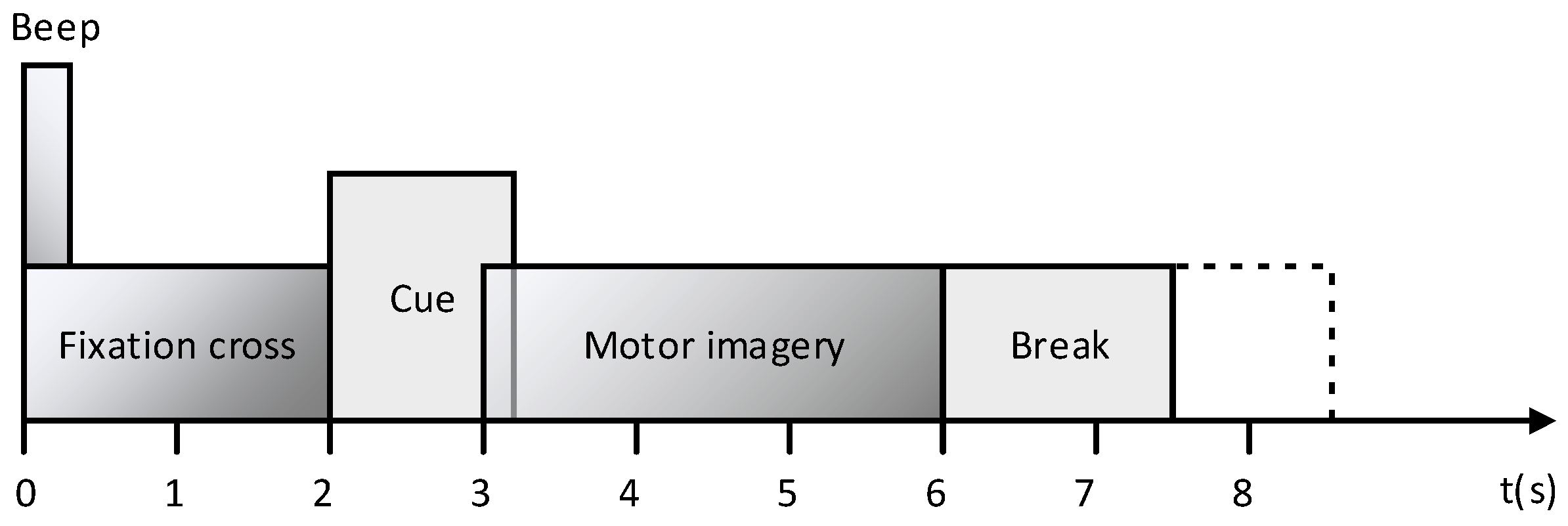
2.1. Dataset
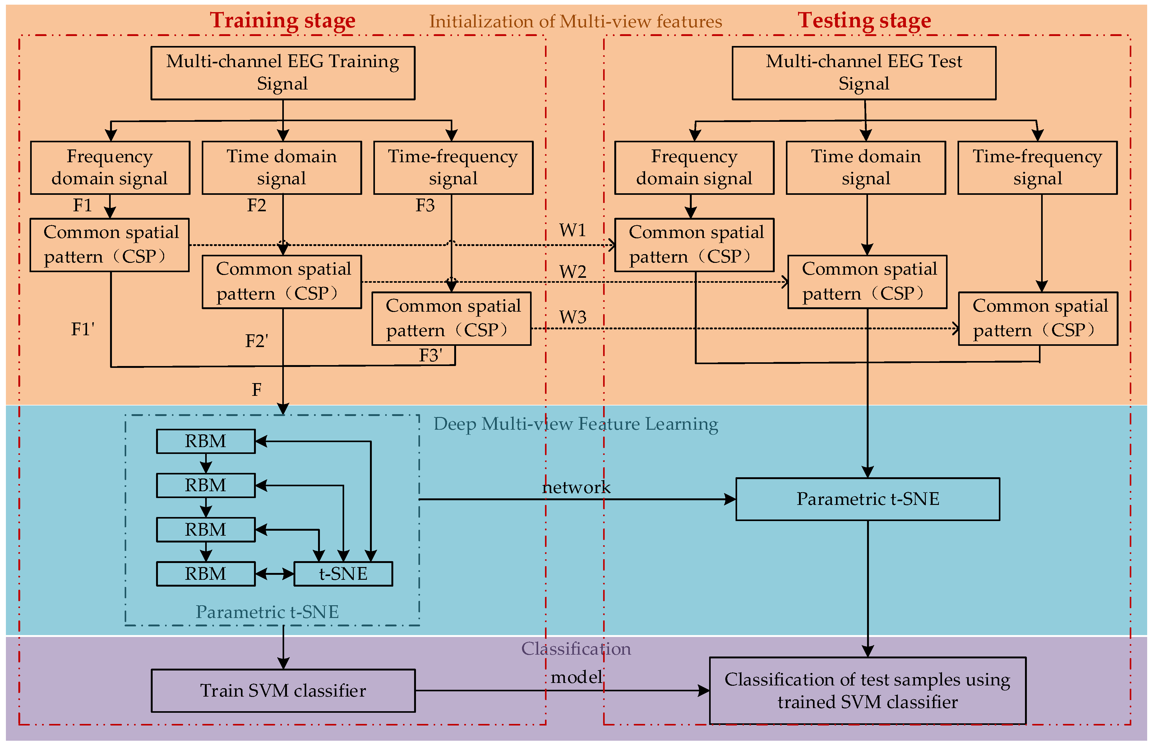
2.2. Initialization of Multi-View Features
2.2.1. Time Domain Features
2.2.2. Frequency Domain Features
2.2.3. Time-Frequency Domain Features
2.2.4. Spatial Domain Features
2.3. Deep Multi-View Feature Learning
2.3.1. Pretraining
2.3.2. Fine-Tuning
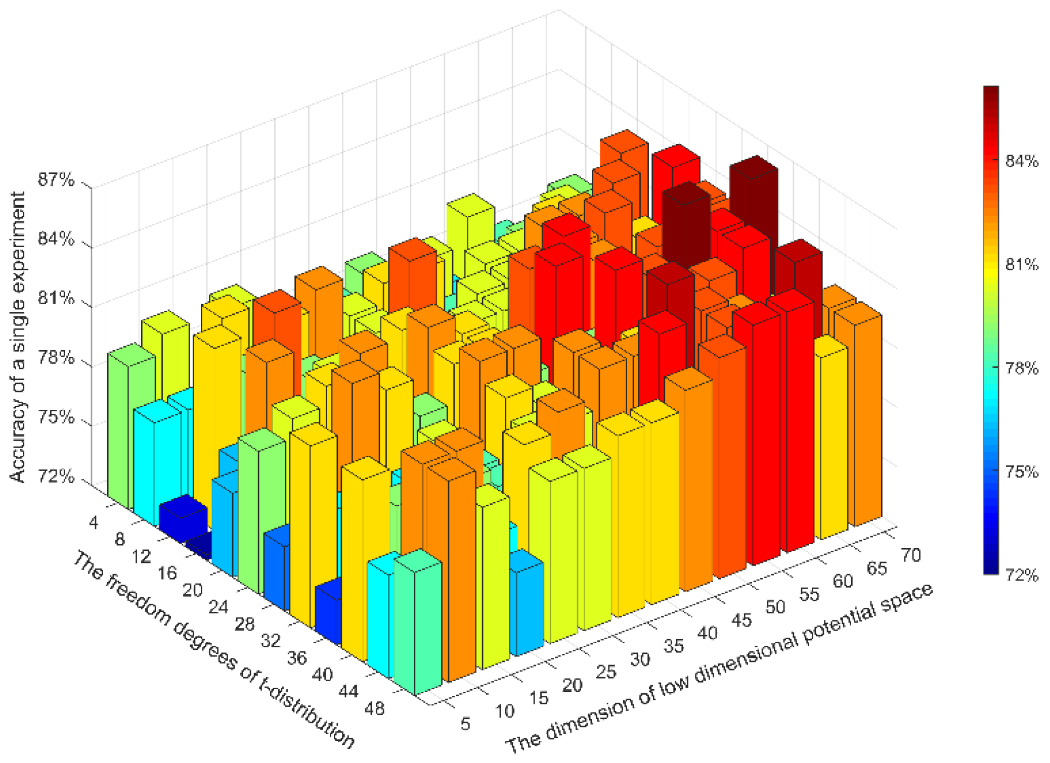
2.4. Optimization of Network Parameters
2.5. The Selection of Classifer Algorithm
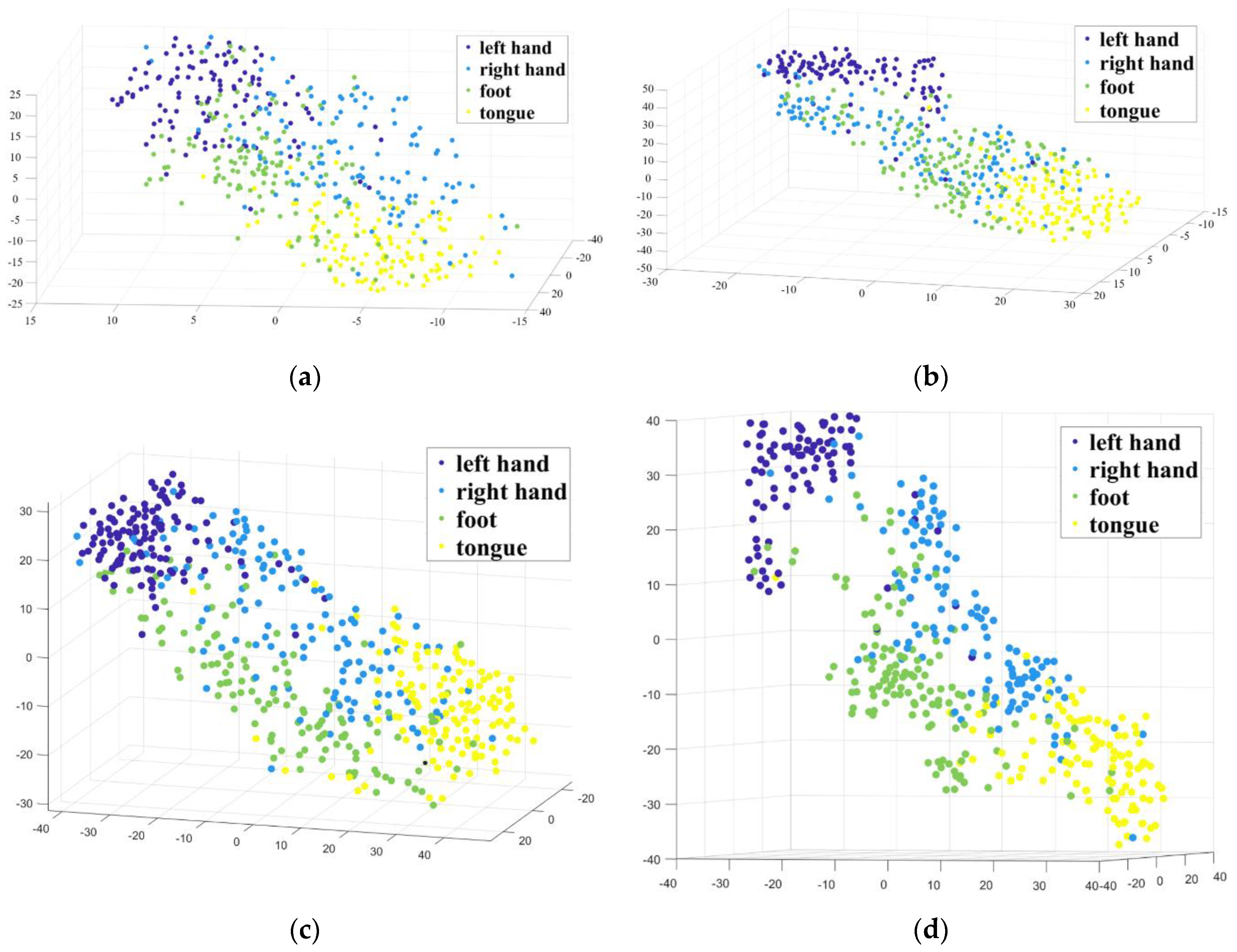
3. Results
4. Discussion
5. Conclusions
Author Contributions
Funding
Conflicts of Interest
References
- Daly, J.J.; Wolpaw, J.R. Brain-computer interfaces in neurological rehabilitation. Lancet Neurol. 2008, 7, 1032–1043. [Google Scholar] [CrossRef]
- Miao, M.; Wang, A.; Liu, F. Application of artificial bee colony algorithm in feature optimization for motor imagery EEG classification. Neural Comput. Appl. 2017, 30, 3677–3691. [Google Scholar] [CrossRef]
- Farahat, A.; Reichert, C.; Sweeney-Reed, C.M.; Hinrichs, H. Convolutional neural networks for decoding of covert attention focus and saliency maps for EEG feature visualization. J. Neural Eng. 2019, 16, 066010. [Google Scholar] [CrossRef] [Green Version]
- Razi, S.; Mollaei, M.R.K.; Ghasemi, J. A novel method for classification of BCI multi-class motor imagery task based on Dempster-Shafer theory. Inf. Sci. 2019, 484, 14–26. [Google Scholar] [CrossRef]
- Mejia Tobar, A.; Hyoudou, R.; Kita, K.; Nakamura, T.; Kambara, H.; Ogata, Y.; Hanakawa, T.; Koike, Y.; Yoshimura, N. Decoding of ankle flexion and extension from cortical current sources estimated from non-invasive brain activity recording methods. Front. Neurosci. 2017, 11, 733. [Google Scholar] [CrossRef] [PubMed]
- Kumar, S.; Sharma, A.; Tsunoda, T. An improved discriminative filter bank selection approach for motor imagery EEG signal classification using mutual information. Bmc Bioinf. 2017, 18, 126–137. [Google Scholar] [CrossRef] [Green Version]
- Li, D.L.; Wang, J.H.; Xu, J.C.; Fang, X.K. Densely Feature Fusion Based on Convolutional Neural Networks for Motor Imagery EEG Classification. IEEE Access 2019, 7, 132720–132730. [Google Scholar] [CrossRef]
- Chin, Z.Y.; Ang, K.K.; Wang, C.C.; Auan, C.T.; Zhang, H.H.; IEEE. Multi-class Filter Bank Common Spatial Pattern for Four-Class Motor Imagery BCI. In Proceedings of the 2009 Annual International Conference of the Ieee Engineering in Medicine and Biology Society, New York, NY, USA, 3–6 September 2009. [Google Scholar]
- Wolpaw, J.R.; Birbaumer, N.; McFarland, D.J.; Pfurtscheller, G.; Vaughan, T.M. Brain-Computer interfaces (BCIs) for communication and control. Suppl. Clin. Neurophysiol. 2004, 57, 607–613. [Google Scholar]
- Ang, K.K.; Guan, C. EEG-based strategies to detect motor imagery for control and rehabilitation. IEEE Trans. Neural Syst. Rehabil. Eng. 2017, 25, 392–401. [Google Scholar] [CrossRef]
- Baig, M.Z.; Aslaml, N.; Shum, H.P.H. Filtering techniques for channel selection in motor imagery EEG applications: A survey. Artif. Intell. Rev. 2020, 53, 1207–1232. [Google Scholar] [CrossRef] [Green Version]
- Mahmoudi, M.; Shamsi, M. Multi-class EEG classification of motor imagery signal by finding optimal time segments and features using SNR-based mutual information. Australas. Phys. Eng. Sci. Med. 2018, 41, 957–972. [Google Scholar] [CrossRef] [PubMed]
- Wang, L.; Liu, X.C.; Liang, Z.W.; Yang, Z.; Hu, X. Analysis and classification of hybrid BCI based on motor imagery and speech imagery. Measurement. 2019, 147, 12. [Google Scholar] [CrossRef]
- Majidov, I.; Whangbo, T. Efficient Classification of Motor Imagery Electroencephalography Signals Using Deep Learning Methods. Sensors 2019, 19. [Google Scholar] [CrossRef] [PubMed] [Green Version]
- Kumar, S.; Sharma, A. A new parameter tuning approach for enhanced motor imagery EEG signal classification. Med. Biol Eng. Comput. 2018, 56, 1861–1874. [Google Scholar] [CrossRef] [PubMed] [Green Version]
- Li, Y.; Zhang, X.R.; Zhang, B.; Lei, M.Y.; Cui, W.G.; Guo, Y.Z. A Channel-Projection Mixed-Scale Convolutional Neural Network for Motor Imagery EEG Decoding. IEEE Trans. Neural Syst. Rehabil. Eng. 2019, 27, 1170–1180. [Google Scholar] [CrossRef]
- Ang, K.K.; Chin, Z.Y.; Zhang, H.H.; Guan, C.T. Filter Bank Common Spatial Pattern (FBCSP) in Brain-Computer Interface. In Proceedings of the 2008 IEEE International Joint Conference on Neural Networks, New York, NY, USA, 8 May 2008; pp. 2390–2397. [Google Scholar]
- Lemm, S.; Blankertz, B.; Curio, G.; Muller, K.R. Spatio-spectral filters for improving the classification of single trial EEG. IEEE Trans. Biomed. Eng. 2005, 52, 1541–1548. [Google Scholar] [CrossRef]
- Dornhege, G.; Blankertz, B.; Krauledat, M.; Losch, F.; Curio, G.; Muller, K.R. Combined optimization of spatial and temporal filters for improving brain-computer interfacing. IEEE Trans. Biomed. Eng. 2006, 53, 2274–2281. [Google Scholar] [CrossRef]
- Novi, Q.; Guan, C.; Dat, T.H.; Xue, P. Sub-band Common Spatial Pattern (SBCSP) for Brain-Computer Interface. In Proceedings of the 2007 3rd International IEEE/EMBS Conference on Neural Engineering, Kohala Coast, HI, USA, 2–5 May 2007; pp. 204–207. [Google Scholar]
- Thomas, K.P.; Guan, C.; Lau, C.T.; Vinod, A.P.; Ang, K.K. A new discriminative common spatial pattern method for motor imagery brain-computer interfaces. IEEE Trans. Biomed. Eng. 2009, 56, 2730–2733. [Google Scholar] [CrossRef]
- Jiang, Y.; Deng, Z.; Chung, F.-L.; Wang, G.; Qian, P.; Choi, K.-S.; Wang, S. Recognition of epileptic EEG signals using a novel multiview TSK fuzzy system. IEEE Trans. Fuzzy Syst. 2017, 25, 3–20. [Google Scholar] [CrossRef]
- Li, J.; Yu, Z.L.; Gu, Z.; Wu, W.; Li, Y.; Jin, L. A hybrid network for ERP detection and analysis based on restricted Boltzmann machine. IEEE Trans. Neural Syst. Rehabil. Eng. 2018, 26, 563–572. [Google Scholar] [CrossRef]
- Li, J.; Yu, Z.L.; Gu, Z.; Tan, M.; Wang, Y.; Li, Y. Spatial-temporal discriminative restricted Boltzmann machine for event-related potential detection and analysis. IEEE Trans. Neural Syst. Rehabil. Eng. 2019, 27, 139–151. [Google Scholar] [CrossRef] [PubMed]
- Lu, N.; Li, T.; Ren, X.; Miao, H. A deep learning scheme for motor imagery classification based on restricted boltzmann machines. IEEE Trans. Neural Syst. Rehabil. Eng. 2017, 25, 566–576. [Google Scholar] [CrossRef] [PubMed]
- Maaten, L.V.D. Learning a parametric embedding by preserving local structure. J. Mach. Learn. Res. 2009, 5, 384–391. [Google Scholar]
- Mohseni, M.; Shalchyan, V.; Jochumsen, M.; Niazi, I.K. Upper limb complex movements decoding from pre-movement EEG signals using wavelet common spatial patterns. Comput. Methods Programs Biomed. 2020, 183, 10. [Google Scholar] [CrossRef]
- Yang, B.; Li, H.; Wang, Q.; Zhang, Y. Subject-based feature extraction by using fisher WPD-CSP in brain-computer interfaces. Comput. Methods Programs Biomed. 2016, 129, 21–28. [Google Scholar] [CrossRef]
- Blankertz, B.; Tomioka, R.; Lemm, S.; Kawanabe, M.; Muller, K.R. Optimizing spatial filters for robust EEG single-trial analysis. IEEE Signal. Process. Mag. 2008, 25, 41–56. [Google Scholar] [CrossRef]
- Miao, M.; Zeng, H.; Wang, A.; Zhao, C.; Liu, F. Discriminative spatial-frequency-temporal feature extraction and classification of motor imagery EEG: An sparse regression and Weighted Naive Bayesian Classifier-based approach. J. Neurosci. Methods 2017, 278, 13–24. [Google Scholar] [CrossRef]
- Nasihatkon, B.; Boostani, R.; Jahromi, M.Z. An efficient hybrid linear and kernel CSP approach for EEG feature extraction. Neurocomputing 2009, 73, 432–437. [Google Scholar] [CrossRef]
- Jafarifarmand, A.; Badamchizadeh, M.A.; Khanmohammadi, S.; Nazari, M.A.; Tazehkand, B.M. A new self-regulated neuro-fuzzy framework for classification of EEG signals in motor imagery BCI. IEEE Trans. Fuzzy Syst. 2018, 26, 1485–1497. [Google Scholar] [CrossRef]
- Li, M.A.; Luo, X.Y.; Yang, J.F. Extracting the nonlinear features of motor imagery EEG using parametric t-SNE. Neurocomputing 2016, 218, 371–381. [Google Scholar] [CrossRef]
- Hinton, G.E.; Salakhutdinov, R.R. Reducing the dimensionality of data with neural networks. Science 2006, 313, 504–507. [Google Scholar] [CrossRef] [PubMed] [Green Version]
- Hinton, G.E.; Osindero, S.; Teh, Y.W. A fast learning algorithm for deep belief nets. Neural Comput. 2006, 18, 1527–1554. [Google Scholar] [CrossRef] [PubMed]
- Hinton, G.; Roweis, S. Stochastic neighbor embedding. In Proceedings of the Advances in Neural Information Processing Systems, Cambridge, MA, USA, 1 October 2003; pp. 833–840. [Google Scholar]
- Laurens, V.D.M.; Hinton, G. Visualizing Data using t-SNE. J. Mach. Learn. Res. 2008, 9, 2579–2605. [Google Scholar]
- He, L.M.; Yang, X.B.; Lu, H.J. A Comparison of Support Vector Machines Ensemble for Classification. In Proceedings of the 2007 International Conference on Machine Learning and Cybernetics, Hong Kong, China, 19–22 August 2007; pp. 3613–3617. [Google Scholar]
- Cortes, C.; Vapnik, V. Support-vector networks. Mach. Learn. 1995, 20, 273–297. [Google Scholar] [CrossRef]
- Dai, M.; Zheng, D.; Na, R.; Wang, S.; Zhang, S. EEG classification of motor imagery using a novel deep learning framework. Sensors 2019, 19, 551. [Google Scholar] [CrossRef] [PubMed] [Green Version]
- Ang, K.K.; Chin, Z.Y.; Wang, C.; Guan, C.; Zhang, H. Filter bank common spatial pattern algorithm on BCI competition IV datasets 2a and 2b. Front. Neurosci. 2012, 6, 39. [Google Scholar] [CrossRef] [PubMed] [Green Version]
- Sakhavi, S.; Guan, C.; Yan, S. Learning temporal information for brain-computer interface using convolutional neural networks. IEEE Trans. Neural Netw Learn. Syst. 2018, 29, 5619–5629. [Google Scholar] [CrossRef]
- Bashashati, H.; Ward, R.K.; Bashashati, A. User-customized brain computer interfaces using Bayesian optimization. J. Neural Eng. 2016, 13, 026001. [Google Scholar] [CrossRef]
- Aghaei, A.S.; Mahanta, M.S.; Plataniotis, K.N. Separable common spatio-spectral patterns for motor imagery BCI systems. IEEE Trans. Biomed. Eng. 2016, 63, 15–29. [Google Scholar] [CrossRef]
- Gaur, P.; Pachori, R.B.; Wang, H.; Prasad, G. A multi-class EEG-based BCI classification using multivariate empirical mode decomposition based filtering and Riemannian geometry. Expert Syst. Appl. 2018, 95, 201–211. [Google Scholar] [CrossRef]
- Olivas-Padilla, B.E.; Chacon-Murguia, M.I. Classification of multiple motor imagery using deep convolutional neural networks and spatial filters. Appl. Soft Comput. 2019, 75, 461–472. [Google Scholar] [CrossRef]
- Zeng, H.; Song, A. Optimizing Single-Trial EEG Classification by Stationary Matrix Logistic Regression in Brain-Computer Interface. IEEE Trans. Neural Netw Learn. Syst 2016, 27, 2301–2313. [Google Scholar] [CrossRef] [PubMed]
- Xie, X.; Yu, Z.L.; Lu, H.; Gu, Z.; Li, Y. Motor imagery classification based on bilinear sub-manifold learning of symmetric positive-definite matrices. IEEE Trans. Neural Syst. Rehabil. Eng. 2017, 25, 504–516. [Google Scholar] [CrossRef] [PubMed] [Green Version]


| Methods | Single-View Time Domain | Single-View Frequency Domain | Single-View Time-Frequency | Multi-View |
|---|---|---|---|---|
| Subject 1 | 75.8929 (0.6786) | 80.3571 (0.7381) | 79.4643 (0.7262) | 86.6071 (0.8214) |
| Subject 2 | 50.4505 (0.3399) | 54.9550 (0.3994) | 52.2523 (0.3635) | 61.2613 (0.4838) |
| Subject 3 | 76.3636 (0.6849) | 80.9091 (0.7454) | 79.0909 (0.7211) | 87.2727 (0.7696) |
| Subject 4 | 58.8000 (0.4506) | 70.8000 (0.6102) | 64.6000 (0.5278) | 75.2000 (0.6664) |
| Subject 5 | 47.2727 (0.2954) | 45.4545 (0.2709) | 50.9091 (0.3439) | 64.5455 (0.5024) |
| Subject 6 | 44.3182 (0.2571) | 48.8636 (0.3179) | 47.7273 (0.3016) | 65.9091 (0.5301) |
| Subject 7 | 77.4775 (0.6995) | 80.1802 (0.7357) | 76.5766 (0.6875) | 83.7838 (0.7837) |
| Subject 8 | 79.8165 (0.7308) | 80.7339 (0.7431) | 75.2294 (0.6697) | 89.9083 (0.8655) |
| Subject 9 | 83.1683 (0.7752) | 82.1782 (0.7620) | 72.2772 (0.6293) | 92.0792 (0.8942) |
| Average | 65.9511 (0.5458) | 69.3812 (0.5914) | 66.4586 (0.5523) | 78.5074 (0.6278) |
| Methods | FBCSP [41] | BO [43] | Monolithic Network [46] | FBCSP-SVM [42] | CW-CNN [42] | SCSSP [44] | DFFN [7] | Proposed Methods |
|---|---|---|---|---|---|---|---|---|
| Subject 1 | 76.00 | 82.12 | 83.13 | 82.29 | 86.11 | 67.88 | 83.20 | 86.6071 |
| Subject 2 | 56.50 | 44.86 | 65.45 | 60.42 | 60.76 | 42.18 | 65.69 | 61.2613 |
| Subject 3 | 81.25 | 86.6 | 80.29 | 82.99 | 86.81 | 77.87 | 90.29 | 87.2727 |
| Subject 4 | 61.00 | 66.28 | 81.60 | 72.57 | 67.36 | 51.77 | 69.42 | 75.2000 |
| Subject 5 | 55.00 | 48.72 | 76.70 | 60.07 | 62.50 | 50.17 | 61.65 | 64.5455 |
| Subject 6 | 45.25 | 53.3 | 71.12 | 44.10 | 45.14 | 45.97 | 60.74 | 65.9091 |
| Subject 7 | 82.75 | 72.64 | 84.00 | 86.11 | 90.63 | 87.5 | 85.18 | 83.7838 |
| Subject 8 | 81.25 | 82.33 | 82.66 | 77.08 | 81.25 | 85.79 | 84.21 | 89.9083 |
| Subject 9 | 70.75 | 76.35 | 80.74 | 75.00 | 77.08 | 76.31 | 85.48 | 92.0792 |
| Average | 67.75 | 68.13 | 78.41 | 71.18 | 73.07 | 65.05 | 76.44 | 78.5074 |
| Methods | SS-MEMDBF [45] | Miao et al. [2] | Monolithic Network [46] | FBCSP-SVM [42] | CW-CNN [42] | sMLR [47] | TSSM-SVM [48] | Proposed Methods |
|---|---|---|---|---|---|---|---|---|
| Subject 1 | 0.86 | 0.6481 | 0.67 | 0.7640 | 0.8150 | 0.7407 | 0.70 | 0.8214 |
| Subject 2 | 0.24 | 0.3657 | 0.35 | 0.4720 | 0.4770 | 0.2685 | 0.32 | 0.4838 |
| Subject 3 | 0.70 | 0.6632 | 0.65 | 0.7730 | 0.8240 | 0.7685 | 0.75 | 0.7696 |
| Subject 4 | 0.68 | 0.5046 | 0.62 | 0.6340 | 0.5650 | 0.4259 | 0.54 | 0.6664 |
| Subject 5 | 0.36 | 0.3241 | 0.58 | 0.4680 | 0.5000 | 0.2870 | 0.32 | 0.5024 |
| Subject 6 | 0.34 | 0.2963 | 0.45 | 0.2550 | 0.2690 | 0.2685 | 0.34 | 0.5301 |
| Subject 7 | 0.66 | 0.7188 | 0.69 | 0.8150 | 0.8750 | 0.7315 | 0.70 | 0.7837 |
| Subject 8 | 0.75 | 0.6354 | 0.70 | 0.6940 | 0.7500 | 0.7685 | 0.69 | 0.8655 |
| Subject 9 | 0.82 | 0.6458 | 0.64 | 0.6670 | 0.6940 | 0.7963 | 0.77 | 0.8942 |
| Average | 0.60 | 0.5336 | 0.59 | 0.6160 | 0.6410 | 0.5617 | 0.571 | 0.6278 |
| Methods | Decision Tree | LDA | KNN | NB | SD | SVM |
|---|---|---|---|---|---|---|
| Subject 1 | 74.5 | 85.4 | 75.3 | 82.7 | 86.3 | 86.6071 |
| Subject 2 | 43.9 | 59.0 | 47.7 | 50.5 | 58.2 | 61.2613 |
| Subject 3 | 78.8 | 86.9 | 77.5 | 85.6 | 89.1 | 87.2727 |
| Subject 4 | 48.8 | 68.2 | 50.6 | 63.9 | 72.4 | 75.2000 |
| Subject 5 | 52.2 | 59.6 | 55.4 | 57.4 | 65.4 | 64.5455 |
| Subject 6 | 44.2 | 65.2 | 53.7 | 62.7 | 65.7 | 65.9091 |
| Subject 7 | 73.2 | 80.3 | 72.4 | 81.2 | 82.1 | 83.7838 |
| Subject 8 | 70.8 | 87.7 | 75.3 | 84.1 | 89.5 | 89.9083 |
| Subject 9 | 75.6 | 81.4 | 77.4 | 77.6 | 88.4 | 92.0792 |
| Average | 54.64 | 74.86 | 65.03 | 71.74 | 77.46 | 78.5074 |
© 2020 by the authors. Licensee MDPI, Basel, Switzerland. This article is an open access article distributed under the terms and conditions of the Creative Commons Attribution (CC BY) license (http://creativecommons.org/licenses/by/4.0/).
Share and Cite
Xu, J.; Zheng, H.; Wang, J.; Li, D.; Fang, X. Recognition of EEG Signal Motor Imagery Intention Based on Deep Multi-View Feature Learning. Sensors 2020, 20, 3496. https://doi.org/10.3390/s20123496
Xu J, Zheng H, Wang J, Li D, Fang X. Recognition of EEG Signal Motor Imagery Intention Based on Deep Multi-View Feature Learning. Sensors. 2020; 20(12):3496. https://doi.org/10.3390/s20123496
Chicago/Turabian StyleXu, Jiacan, Hao Zheng, Jianhui Wang, Donglin Li, and Xiaoke Fang. 2020. "Recognition of EEG Signal Motor Imagery Intention Based on Deep Multi-View Feature Learning" Sensors 20, no. 12: 3496. https://doi.org/10.3390/s20123496