Real-Time Prediction of Rate of Penetration in S-Shape Well Profile Using Artificial Intelligence Models


Abstract
1. Introduction
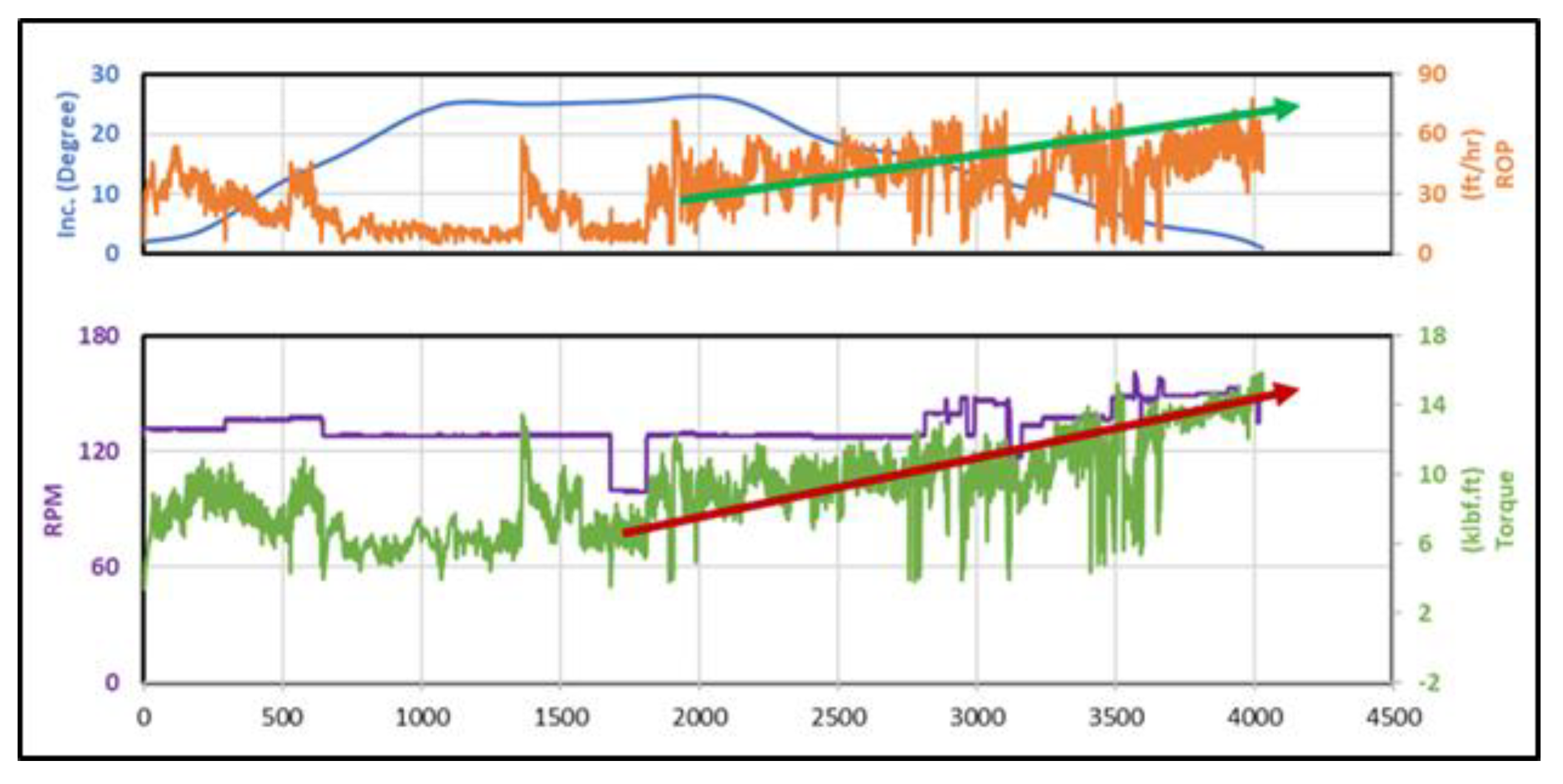
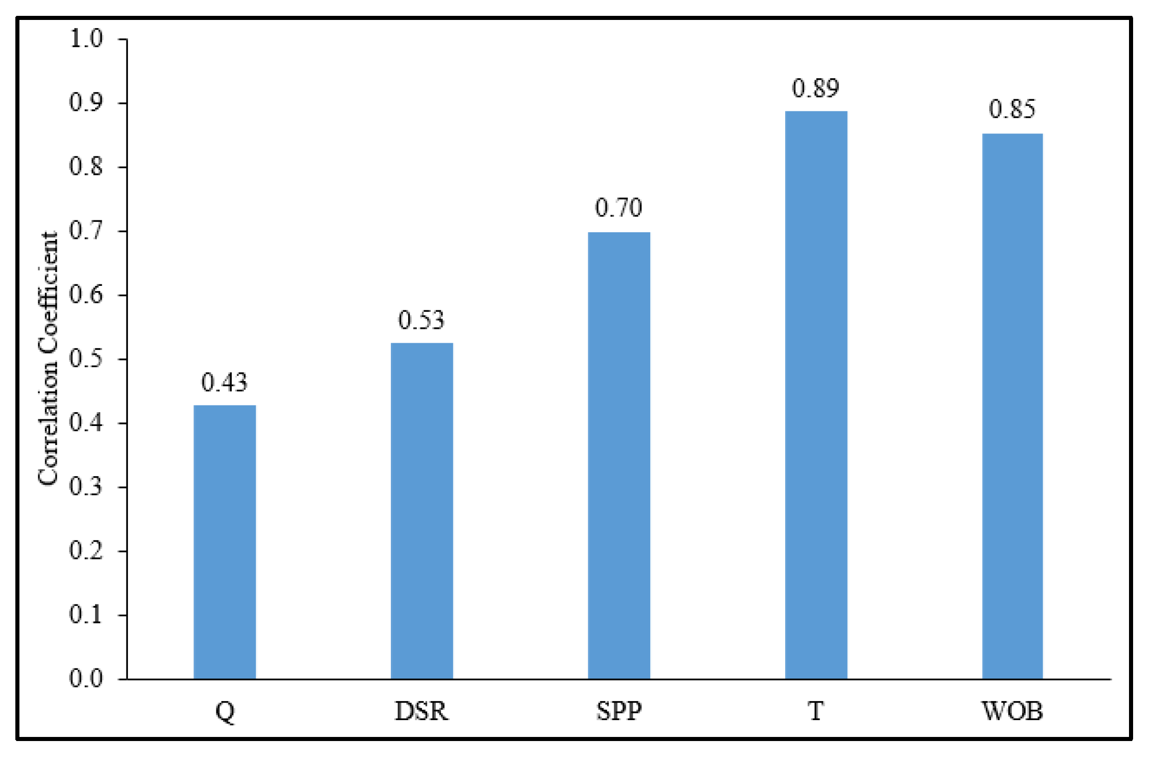
Effect of Drilling Parameters on the Rate of Penetration
2. Artificial Intelligence Models Theory
3. Data Overview and Preparation
4. Artificial Intelligence Models Optimization
5. Results and Discussion
5.1. Training the Artificial Intelligence Models
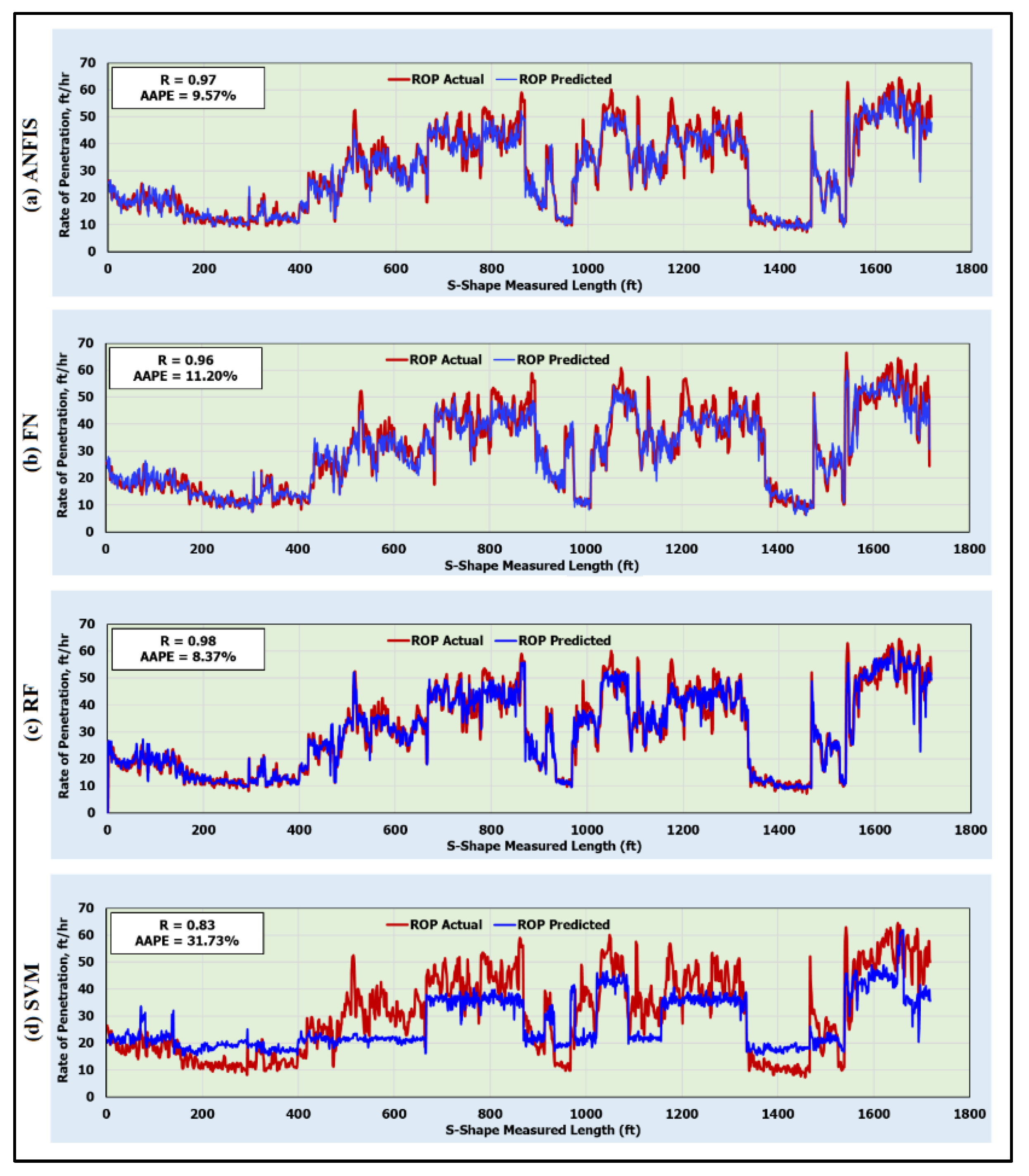
5.2. Testing Artificial Intelligence Models
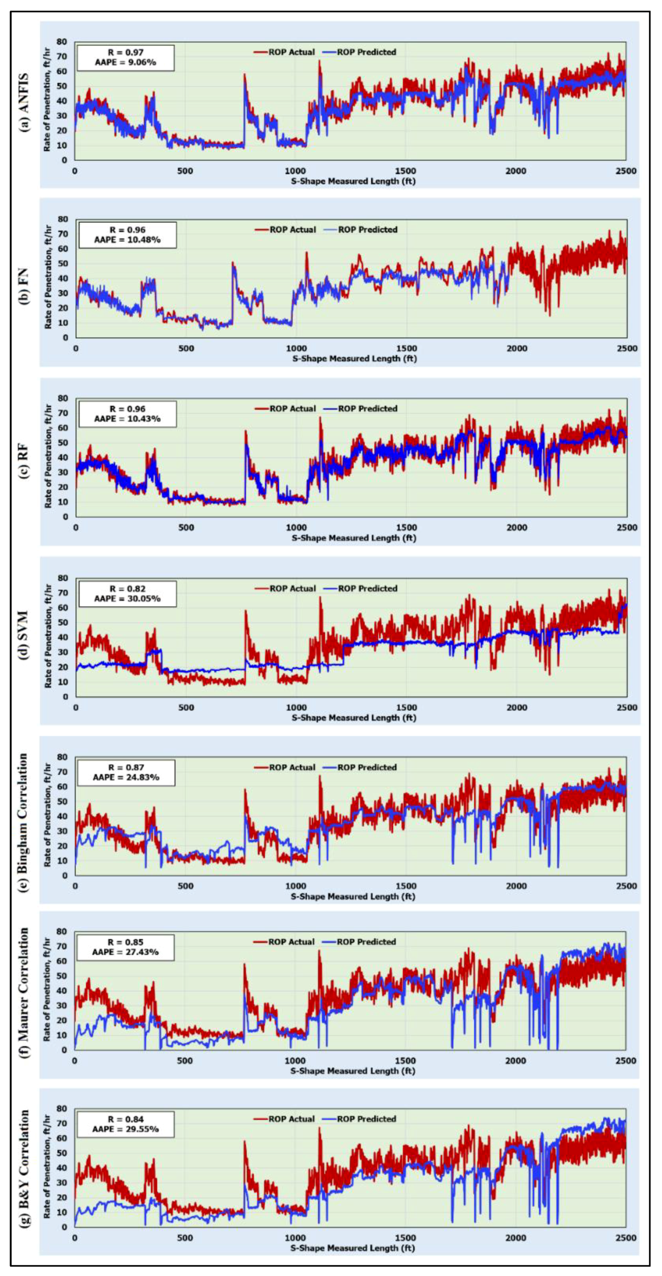
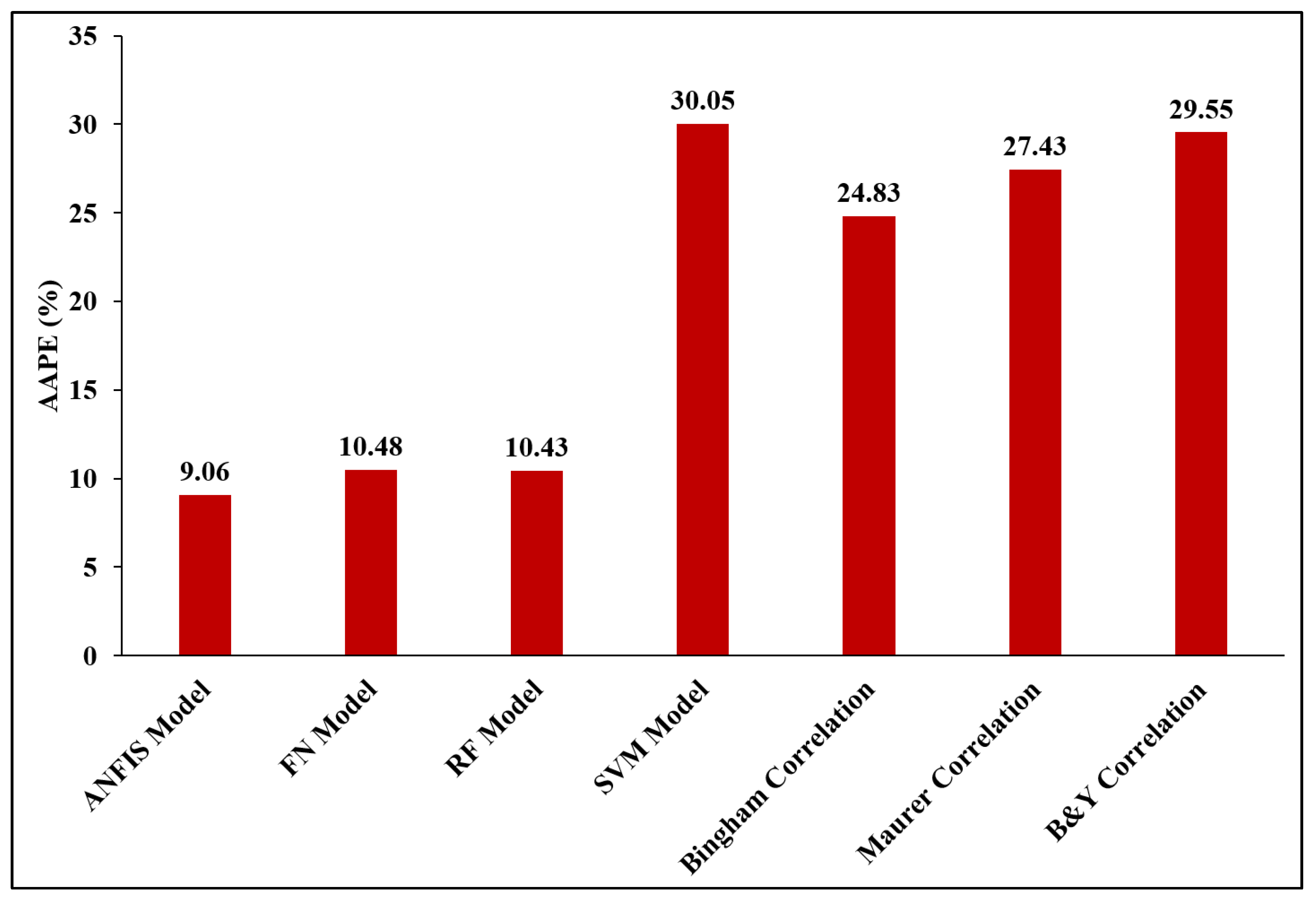
5.3. Validating the Artificial Intelligence Models and Comparison with the Published ROP Correlations
6. Conclusions
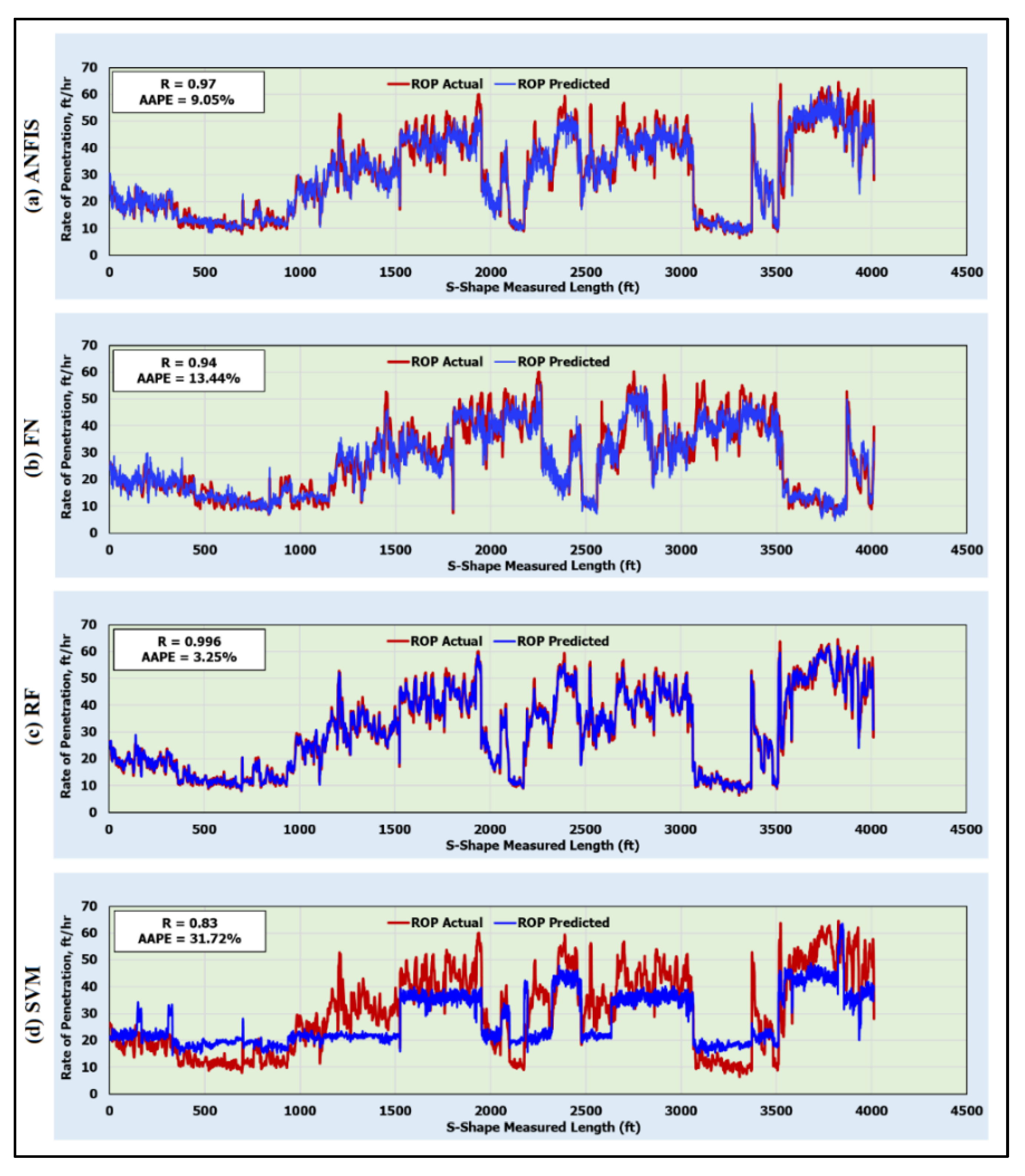
- The ANFIS, FN, and RF models could effectively predict the ROP from the drilling parameters in the S-shape well profile for training, testing, and validation data, whereas the SVM model showed very low accuracy in estimating the ROP.
- The developed ANFIS, FN, and RF models predicted the ROP with AAPEs of 9.50%, 13.44%, and 3.25%, respectively, for the training data.
- For the testing data, the optimized ANFIS, FN, RF models estimated the ROP with AAPEs of 9.57%, 11.20%, and 8.37%, respectively.
- The developed ANFIS, FN, and RF models outperformed the SVM model and the three published empirical correlations for estimating the ROP for the validation data.
Funding
Conflicts of Interest
Abbreviations
| ANN | Artificial neural networks |
| AAPE | Average absolute percentage error |
| AI | Artificial intelligence |
| BHA | Bottom hole assembly |
| FN | Functional neural networks |
| GPM | Gallon per minute |
| GR | Gamma ray |
| LWD | Logging while drilling |
| MD | Measured depth |
| MW | Mud weight |
| MWD | Measurement while drilling |
| MFV | Marsh funnel viscosity |
| PV | Plastic viscosity |
| Q | Flow rate |
| R | Correlation coefficient |
| RF | Random forests |
| RMSE | Root mean square error |
| ROP | Rate of penetration |
| DSR | Drillstring rotation |
| SaDE | Self-adaptive differential evolution |
| SPP | Standpipe pressure |
| SVM | Support vector machine |
| TFA | Total flow area |
| TVD | True vertical depth |
| UCS | Unconfined compressive strength |
| WOB | Weight on bit |
Appendix A
Appendix B

| Reference | Method | Input Parameters | Formula | Constants |
|---|---|---|---|---|
| Maurer [14] | Empirical | DSR, WOB, bit size, uniaxial compressive strength (UCS) | K = 60,087 × 103 | |
| Bingham [15] | Empirical | DSR, WOB, bit size | K = 1.04; a = 0.081; c = 1.08 | |
| Bourgoyne and Young’s [16] | Empirical | True vertical depth (TVD), mud weight (MW), pore pressure, WOB, DSR, bit wear, Q, TFA | a1 = 14.35; a2 = −1.5 × 10⁻³; a3 = −9 × 10⁻⁴; a4 = 3 × 10⁻⁴; a5 = 1.496; a6 = 1.269; a7 = 0.118 | |
| Warren [17] | Empirical | WOB, DSR, bit size, UCS | ||
| Osgouei [4] | Empirical | TVD, MW, pore pressure, WOB, DSR, bit wear, Q, TFA, bit type, inclination | ||
| Al-AbdulJabbar [18] | Empirical | DSR, WOB, torque, SPP, Q, bit size, UCS, MW, drilling fluid plastic viscosity (PV) | ||
| Elkatatny et al. [41] | ANN | Q, SPP, DSR, WOB, MW, torque, PV | - | |
| Al-AbdulJabbar et al. [31] | ANN | WOB, DSR, SPP, Q, torque | - | |
| Ahmed et al. [33] | SVM | Q, SPP, DSR, WOB, MW, torque, drilling fluid yield point, marsh funnel viscosity, PV, solids volume | - | |
| Al-AbdulJabbar et al. [34] | ANN SaDE | DSR, torque, WOB, GR, formation deep resistivity, formation bulk density | - |
Appendix C
| S-Shape Measured Length (ft) | Inputs | Actual ROP, ft/hr | * Empirical Correlations-Based ROP, ft/hr | AI-Based ROP, ft/hr | |||||||||||||
|---|---|---|---|---|---|---|---|---|---|---|---|---|---|---|---|---|---|
| GPM | RPM | WOB, Klbf | Torque, Klbf-ft | SPP, psi | Density, PCF | Bit Size, in | PV | UCS, psi | Bingham [15] | Maurer [14] | B&Y [16] | ANFIS | FN | RF | SVM | ||
| 116 | 843.91 | 131 | 32.46 | 10.4 | 1715.77 | 67 | 12 | 30 | 35,000 | 36.04 | 32.06 | 23.04 | 16.77 | 36.75 | 36.84 | 36.63 | 23.42 |
| 133 | 848.33 | 132 | 31 | 9.88 | 1704.99 | 67 | 12 | 30 | 35,000 | 34.24 | 30.81 | 21.17 | 15.87 | 33.91 | 32.81 | 36.62 | 22.52 |
| 165 | 838.79 | 131 | 32.81 | 8.03 | 1667.65 | 67 | 12 | 30 | 35,000 | 26.02 | 32.42 | 23.54 | 17.21 | 26.43 | 23.76 | 28.26 | 22.02 |
| 241 | 843.76 | 136 | 26.39 | 7.32 | 1708.81 | 67 | 12 | 30 | 25,000 | 19.25 | 26.93 | 15.81 | 13.36 | 19.95 | 18.55 | 20.22 | 21.74 |
| 244 | 841.18 | 136 | 26.26 | 8.29 | 1706.76 | 67 | 12 | 30 | 25,000 | 24.22 | 26.79 | 15.65 | 13.27 | 24.25 | 22.99 | 25.14 | 21.88 |
| 249 | 844.89 | 137 | 25.79 | 7.82 | 1697.29 | 67 | 12 | 30 | 25,000 | 17.88 | 26.50 | 15.21 | 13.05 | 17.88 | 20.40 | 20.89 | 21.28 |
| 254 | 845.49 | 136 | 26.66 | 7.74 | 1681.81 | 67 | 12 | 30 | 25,000 | 20.69 | 27.21 | 16.13 | 13.60 | 20.82 | 20.02 | 20.65 | 20.93 |
| 288 | 844.31 | 136 | 27.62 | 7.31 | 1675.32 | 67 | 12 | 30 | 25,000 | 19.61 | 28.23 | 17.32 | 14.48 | 18.64 | 18.45 | 20.11 | 20.96 |
| 306 | 843.33 | 136 | 27.67 | 8.26 | 1690.02 | 67 | 12 | 30 | 25,000 | 22.85 | 28.28 | 17.38 | 14.57 | 23.89 | 23.03 | 23.11 | 21.56 |
| 362 | 940.81 | 137 | 27.31 | 8.2 | 2027.27 | 67 | 12 | 30 | 30,000 | 23.07 | 28.12 | 17.05 | 14.86 | 24.13 | 24.57 | 23.63 | 28.72 |
| 365 | 948.98 | 138 | 27.66 | 8.34 | 2050.49 | 67 | 12 | 30 | 30,000 | 23.5 | 28.72 | 17.62 | 15.31 | 23.12 | 25.55 | 22.02 | 29.39 |
| 388 | 917.14 | 136 | 28.79 | 6.57 | 1961.94 | 67 | 12 | 30 | 30,000 | 18.09 | 29.47 | 18.81 | 15.97 | 17.52 | 17.83 | 18.86 | 27.45 |
| 1076 | 698.38 | 128 | 31.46 | 8.3 | 1371.99 | 67 | 12 | 30 | 25,000 | 27.61 | 30.27 | 21.14 | 19.81 | 26.69 | 25.08 | 26.23 | 21.28 |
| 1326 | 892.46 | 128 | 41.82 | 8.5 | 2077.77 | 67 | 12 | 30 | 25,000 | 35.83 | 40.66 | 37.36 | 33.28 | 37.25 | 35.17 | 36.01 | 36.55 |
| 1488 | 898.03 | 128 | 38.49 | 7.95 | 2065.37 | 67 | 12 | 30 | 25,000 | 33.81 | 37.31 | 31.65 | 30.48 | 33.70 | 30.70 | 34.64 | 34.88 |
| 1720 | 887.69 | 128 | 30.47 | 11.38 | 2040.27 | 67 | 12 | 30 | 25,000 | 42.82 | 29.28 | 19.84 | 22.41 | 40.92 | 46.10 | 43.66 | 32.95 |
| 1723 | 890.21 | 140 | 34.16 | 10.45 | 2060.76 | 67 | 12 | 30 | 25,000 | 44.91 | 36.31 | 27.27 | 29.83 | 44.08 | 43.12 | 48.13 | 34.97 |
| 1729 | 891.19 | 140 | 35.53 | 10.89 | 2048.1 | 67 | 12 | 30 | 25,000 | 49.96 | 37.82 | 29.50 | 31.67 | 48.33 | 46.20 | 54.55 | 34.72 |
| 1827 | 856.28 | 128 | 36.48 | 9.27 | 2058.21 | 67 | 12 | 30 | 25,000 | 37.92 | 35.29 | 28.43 | 29.95 | 36.92 | 37.98 | 37.87 | 36.65 |
| 1831 | 851.57 | 146 | 37.61 | 9.47 | 2075.92 | 67 | 12 | 30 | 25,000 | 48.23 | 41.97 | 34.47 | 37.20 | 46.08 | 41.28 | 47.47 | 38.81 |
References
- Bourgoyne, A.T., Jr.; Millheim, K.K.; Chenevert, M.E.; Young, F.S. Applied Drilling Engineering; Society of Petroleum Engineers: Houston, TX, USA, 1986; Volume 1. [Google Scholar]
- Akgun, F. How to Estimate the Maximum Achievable Drilling Rate without Jeopardizing Safety. Soc. Pet. Eng. 2002. [Google Scholar] [CrossRef]
- Hossain, M.E.; Al-Majed, A.A. Fundamentals of Sustainable Drilling Engineering; John Wiley & Sons, Inc.: Hoboken, NJ, USA, 2015. [Google Scholar] [CrossRef]
- Osgouei, R.E. Rate of Penetration Estimation Model for Directional and Horizontal Wells; The Graduate School, Middle East Technical University: Ankara, Turkey, 2007. [Google Scholar]
- Lyons, W.; Gary JPlisga, B.; Lorenz, M. Standard Handbook of Petroleum and Natural Gas Engineering; Gulf Professional Publishing; Elsevier: Amsterdam, The Netherlands, 2004. [Google Scholar]
- Mitchell, R.F.; Miska, S.Z. Fundamentals of Drilling Engineering; Society of Petroleum Engineers: Richardson, TX, USA, 2011. [Google Scholar]
- Hegde, C.; Daigle, H.; Millwater, H.; Gray, K. Analysis of rate of penetration (ROP) prediction in drilling using physics-based and data-driven models. J. Pet. Sci. Eng. 2017, 159, 295–306. [Google Scholar] [CrossRef]
- Ricardo, J.; Mendes, P.; Fonseca, T.C.; Serapaio, A.B.S. Applying a Neuro-model Reference Adaptive Controller in Drilling Optimization. World Oil Magazine, 1 October 2007; Volume 228, 29–38. [Google Scholar]
- Allouche, E.N.; Ariaratnam, S.T.; Lueke, J.S. Horizontal directional drilling: Profile of an emerging industry. J. Constr. Eng. Manag. 2000, 126, 68–76. [Google Scholar] [CrossRef]
- Short, J.A. Introduction to Directional and Horizontal Drilling; Pennwell Corporation: Tulsa, OK, USA, 1993. [Google Scholar]
- Inglis, T. Directional Drilling; Springer Science & Business Media: Berlin, Germany, 2013. [Google Scholar] [CrossRef]
- Rabia, H. Well Engineering and Construction; Entrac Consulting: London, UK, 2001. [Google Scholar]
- Mahmoud, A.A.; Elzenary, M.; Elkatatny, S. New Hybrid Hole Cleaning Model for Vertical and Deviated Wells. J. Energy Resour. Technol. 2020, 142, 034501. [Google Scholar] [CrossRef]
- Maurer, W. The “Perfect—Cleaning” Theory of Rotary Drilling. J. Pet. Technol. 1962, 14, 1270–1274. [Google Scholar] [CrossRef]
- Bingham, M.G. A New Approach to Interpreting Rock Drillability; Petroleum Publishing Co.: Houston, TX, USA, 1965. [Google Scholar]
- Bourgoyne, A.T.; Young, F.S. A Multiple Regression Approach to Optimal Drilling and Abnormal Pressure Detection. Soc. Pet. Eng. J. 1974, 14, 371–384. [Google Scholar] [CrossRef]
- Warren, T.M. Penetration Rate Performance of Roller Cone Bits. Soc. Pet. Eng. J. 1987. [Google Scholar] [CrossRef]
- Al-AbdulJabbar, A.M. Utilizing Field Data to Understand the Effect of Drilling Parameters and Mud Rheology on Rate of Penetration in Carbonate Formations. King Fahd University of Petroleum & Minerals (KFUPM). 2017. Available online: https://eprints.kfupm.edu.sa/id/eprint/140167 (accessed on 25 February 2020).
- Mahmoud, A.A.; Elkatatny, S.; Al-Shehri, D. Application of Machine Learning in Evaluation of the Static Young’s Modulus for Sandstone Formations. Sustainability 2020, 12, 1880. [Google Scholar] [CrossRef]
- Mahmoud, A.A.; Elkatatny, S.; Chen, W.; Abdulraheem, A. Estimation of Oil Recovery Factor for Water Drive Sandy Reservoirs through Applications of Artificial Intelligence. Energies 2019, 12, 3671. [Google Scholar] [CrossRef]
- Mahmoud, A.A.; Elkatatny, S.; Mahmoud, M.; Abouelresh, M.; Abdulraheem, A.; Ali, A. Determination of the total organic carbon (TOC) based on conventional well logs using artificial neural network. Int. J. Coal Geol. 2017, 179, 72–80. [Google Scholar] [CrossRef]
- Ahmed, S.A.; Mahmoud, A.A.; Elkatatny, S. Fracture Pressure Prediction Using Radial Basis Function. In Proceedings of the AADE National Technical Conference and Exhibition, AADE-19-NTCE-061, Denver, CO, USA, 9–10 April 2019. [Google Scholar]
- Mahmoud, A.A.; Elkatatny, S.; Abdulraheem, A.; Mahmoud, M.; Ibrahim, O.; Ali, A. New Technique to Determine the Total Organic Carbon Based on Well Logs Using Artificial Neural Network (White Box). In Proceedings of the 2017 SPE Kingdom of Saudi Arabia Annual Technical Symposium and Exhibition, Dammam, Saudi Arabia, 24–27 April 2017. Paper SPE-188016-MS. [Google Scholar] [CrossRef]
- Ahmed, S.A.; Mahmoud, A.A.; Elkatatny, S.; Mahmoud, M.; Abdulraheem, A. Prediction of Pore and Fracture Pressures Using Support Vector Machine. In Proceedings of the International Petroleum Technology Conference, Beijing, China, 26–28 March 2019. IPTC-19523-MS. [Google Scholar] [CrossRef]
- Elkatatny, S.; Al-AbdulJabbar, A.; Mahmoud, A.A. New Robust Model to Estimate the Formation Tops in Real-Time Using Artificial Neural Networks (ANN). Petrophysics 2019, 60, 825–837. [Google Scholar] [CrossRef]
- Mahmoud, A.A.; Elkatatny, S.; Ali, A.; Abouelresh, M.; Abdulraheem, A. Evaluation of the Total Organic Carbon (TOC) Using Different Artificial Intelligence Techniques. Sustainability 2019, 11, 5643. [Google Scholar] [CrossRef]
- Mahmoud, A.A.; Elkatatny, S.; Ali, A.; Moussa, T. Estimation of Static Young’s Modulus for Sandstone Formation Using Artificial Neural Networks. Energies 2019, 12, 2125. [Google Scholar] [CrossRef]
- Bilgesu, H.; Tetrick, L.; Altmis, U.; Mohaghegh, S.; Ameri, S. A new approach for the prediction of rate of penetration (ROP) values. In Proceedings of the SPE Eastern Regional Meeting, Lexington, Kentucky, 22–24 October 1997. SPE-39231-MS. [Google Scholar] [CrossRef]
- Amar, K.; Ibrahim, A. Rate of penetration prediction and optimization using advances in artificial neural networks, a comparative study. In Proceedings of the 4th International Joint Conference on Computational Intelligence, Barcelona, Spain, 5–7 October 2012; pp. 647–652. [Google Scholar] [CrossRef]
- Elkatatny, S. New Approach to Optimize the Rate of Penetration Using Artificial Neural Network. Arabian J. Sci. Eng. 2017, 43, 6297–6304. [Google Scholar] [CrossRef]
- Al-AbdulJabbar, A.; Elkatatny, S.; Mahmoud, M.; Abdulraheem, A. Predicting Rate of Penetration Using Artificial Intelligence Techniques. In Proceedings of the SPE Kingdom of Saudi Arabia Annual Technical Symposium and Exhibition, Dammam, Saudi Arabia, 23–26 April 2018. [Google Scholar] [CrossRef]
- Elkatatny, S.; Tariq, Z.; Mahmoud, M. Real time prediction of drilling fluid rheological properties using Artificial Neural Networks visible mathematical model (white box). J. Pet. Sci. Eng. 2016, 146, 1202–1210. [Google Scholar] [CrossRef]
- Ahmed, A.S.; Elkatatny, S.; Abdulraheem, A.; Mahmoud, M.; Ali, A.Z.; Mohamed, I.M. Prediction of Rate of Penetration of Deep and Tight Formation Using Support Vector Machine. In Proceedings of the SPE Kingdom of Saudi Arabia Annual Technical Symposium and Exhibition, Dammam, Saudi Arabia, 23–26 April 2018. [Google Scholar] [CrossRef]
- Al-AbdulJabbar, A.; Elkatatny, S.; Mahmoud, A.A.; Moussa, T.; Al-Shehri, D.; Abughaban, M.; Al-Yami, A. Prediction of the rate of penetration while drilling horizontal carbonate reservoirs using the self-adaptive artificial neural networks technique. Sustainability 2020, 12, 1376. [Google Scholar] [CrossRef]
- Jang, R. ANFIS Adaptive Network Based Fuzzy Inference System. IEEE Trans. Syst. Man Cybern. 1993, 23. [Google Scholar] [CrossRef]
- Bello, O.; Asafa, T. A Functional Networks Softsensor for Flowing Bottomhole Pressures and Temperatures in Multiphase Production Wells. In Proceeding of the SPE Intelligent Energy Conference & Exhibition, Utrecht, The Netherlands, 1–3 April 2014. [Google Scholar] [CrossRef]
- Anifowose, F.; Abdulraheem, A. Fuzzy logic-driven and SVM-driven hybrid computational intelligence models applied to oil and gas reservoir characterization. J. Nat. Gas Sci. Eng. 2011, 3, 505–517. [Google Scholar] [CrossRef]
- Zhang, C.; Ma, Y. Ensemble Machine Learning; Springer: Boston, MA, USA, 2012. [Google Scholar]
- Hedge, C.; Wallace, S.; Gray, K. Using Trees, Bagging, and Random Forest to Predict Rate of Penetration during Drilling. In Proceeding of the SPE Middle East Intelligence Oil and Gas Conference and Exhibition, Dubai, UAE, 15–16 September 2015. SPE-176792-MS. [Google Scholar] [CrossRef]
- Rui, J.; Zhang, H.; Zhang, D.; Han, F.; Guo, Q. Total organic carbon content prediction based on support-vector-regression machine with particle swarm optimization. J. Pet. Sci. Eng. 2019, 180, 699–706. [Google Scholar] [CrossRef]
- Elkatatny, S.M.; Tariq, Z.; Mahmoud, M.A.; Al-AbdulJabbar, A. Optimization of Rate of Penetration using Artificial Intelligent Techniques. In Proceedings of the 51st U.S. Rock Mechanics/Geomechanics Symposium, San Francisco, CA, USA, 25–28 June 2017; ARMA-2017-0429. Available online: https://www.onepetro.org/download/conference-paper/ARMA-2017-0429?id=conference-paper%2FARMA-2017-0429 (accessed on 20 January 2020).


| Parameter | Q (gpm) | DSR (rpm) | SPP (psi) | T (klbf-ft) | WOB (klbf) | ROP (ft/h) |
|---|---|---|---|---|---|---|
| Minimum | 559 | 99 | 912 | 4.11 | 5.14 | 6.34 |
| Maximum | 993 | 159 | 2490 | 15.9 | 57.2 | 64.5 |
| Range | 434 | 60 | 1579 | 11.8 | 52.1 | 58.1 |
| Standard deviation | 94.0 | 10.8 | 347 | 2.26 | 11.4 | 15.0 |
| Skewness | −0.596 | −0.976 | −0.349 | 0.524 | 0.045 | 0.184 |
| Kurtosis | −0.692 | 2.643 | −0.952 | −0.140 | −0.941 | −1.193 |
| ANFIS | |
|---|---|
| Cluster radius | 0.1 |
| Ep-size | 300 |
| FN | |
| Training method | Nonlinear function without iteration terms |
| Training function type | Forward selection method |
| RF | |
| Maximum depth | 29 |
| Maximum feature | Sqrt |
| SVM | |
| Kernel | Radial basis function |
| Gamma | Scale |
| No. of iterations | 1000 |
| C | 100 |
| Training | Testing | Validation | ||||
|---|---|---|---|---|---|---|
| R | AAPE % | R | AAPE % | R | AAPE % | |
| Without inclination | 0.97 | 9.05 | 0.97 | 9.57 | 0.97 | 9.06 |
| With inclination | 0.94 | 12.85 | 0.92 | 13.81 | 0.16 | 51.29 |
© 2020 by the author. Licensee MDPI, Basel, Switzerland. This article is an open access article distributed under the terms and conditions of the Creative Commons Attribution (CC BY) license (http://creativecommons.org/licenses/by/4.0/).
Share and Cite
Elkatatny, S. Real-Time Prediction of Rate of Penetration in S-Shape Well Profile Using Artificial Intelligence Models. Sensors 2020, 20, 3506. https://doi.org/10.3390/s20123506
Elkatatny S. Real-Time Prediction of Rate of Penetration in S-Shape Well Profile Using Artificial Intelligence Models. Sensors. 2020; 20(12):3506. https://doi.org/10.3390/s20123506
Chicago/Turabian StyleElkatatny, Salaheldin. 2020. "Real-Time Prediction of Rate of Penetration in S-Shape Well Profile Using Artificial Intelligence Models" Sensors 20, no. 12: 3506. https://doi.org/10.3390/s20123506
APA StyleElkatatny, S. (2020). Real-Time Prediction of Rate of Penetration in S-Shape Well Profile Using Artificial Intelligence Models. Sensors, 20(12), 3506. https://doi.org/10.3390/s20123506