A Method of Multiple Dynamic Objects Identification and Localization Based on Laser and RFID


 ,
,  ,
,
Abstract
:1. Introduction
- (1)
- We present a solution that incorporates RFID phase information and laser range measurements for multiple dynamic objects identification and localization in indoor environments.
- (2)
- We propose incorporating the Pearson correlation coefficient into the update stage of particle filtering. This method can effectively estimate the historical trajectories of moving objects in an environment with obstacles.
- (3)
- We set up different paths in different environments on campus, and thoroughly evaluated our method. Our method can effectively identify and locate the passing pedestrians in indoor scenes when compared to the Bray–Curtis (BC) similarity matching-based approach as well as the particle filter-based approach.
2. Related Work
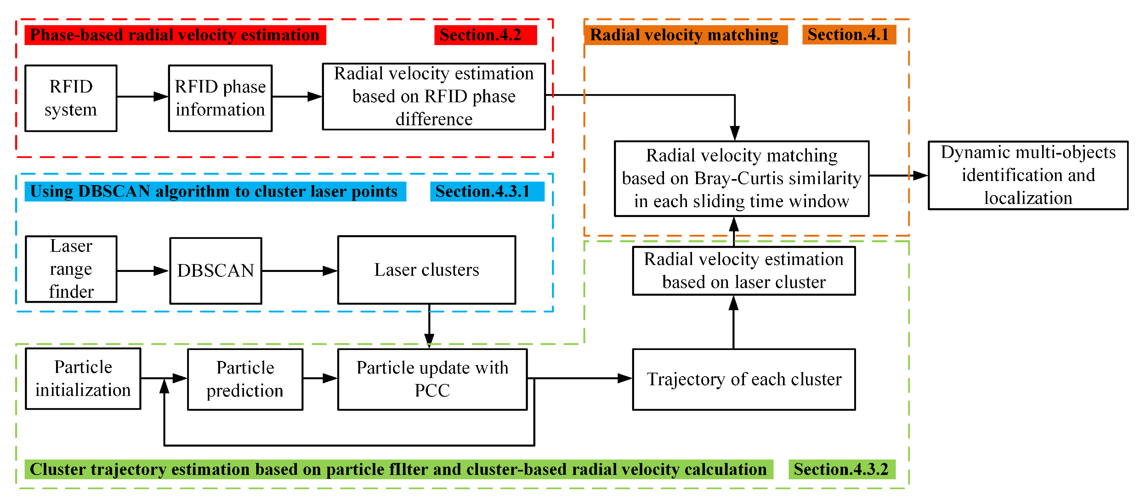
3. System Overview
4. Indoor Multiple Dynamic Objects Identification and Localization
4.1. Object Identification and Localization Based on Radial Velocity Matching
4.2. Estimating the Radial Velocities of Moving Tags Based on RFID Phase Difference
4.3. Estimiating the Radial Velocities of Laser Clusters
4.3.1. Laser Clustering Based on DBSCAN
4.3.2. Cluster Trajectory Estimation Based on Particle Filter
- Prediction
- Update
4.3.3. Calculating Each Cluster’s Radial Velocity
5. Experimental Results Analysis
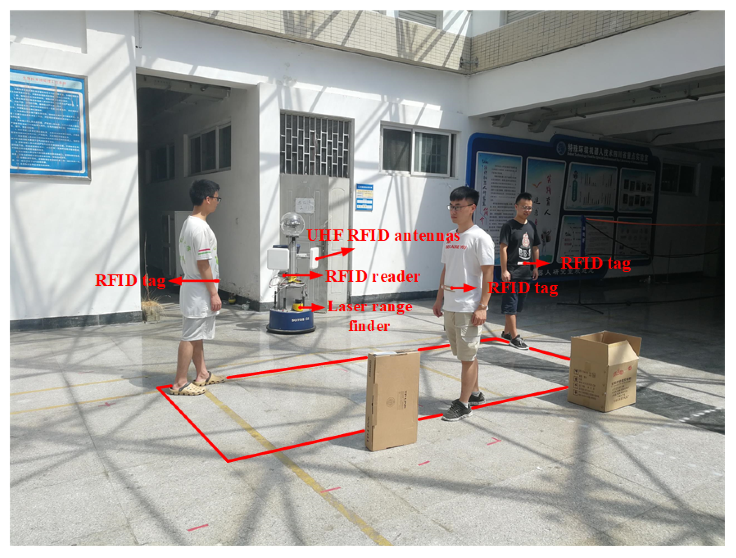
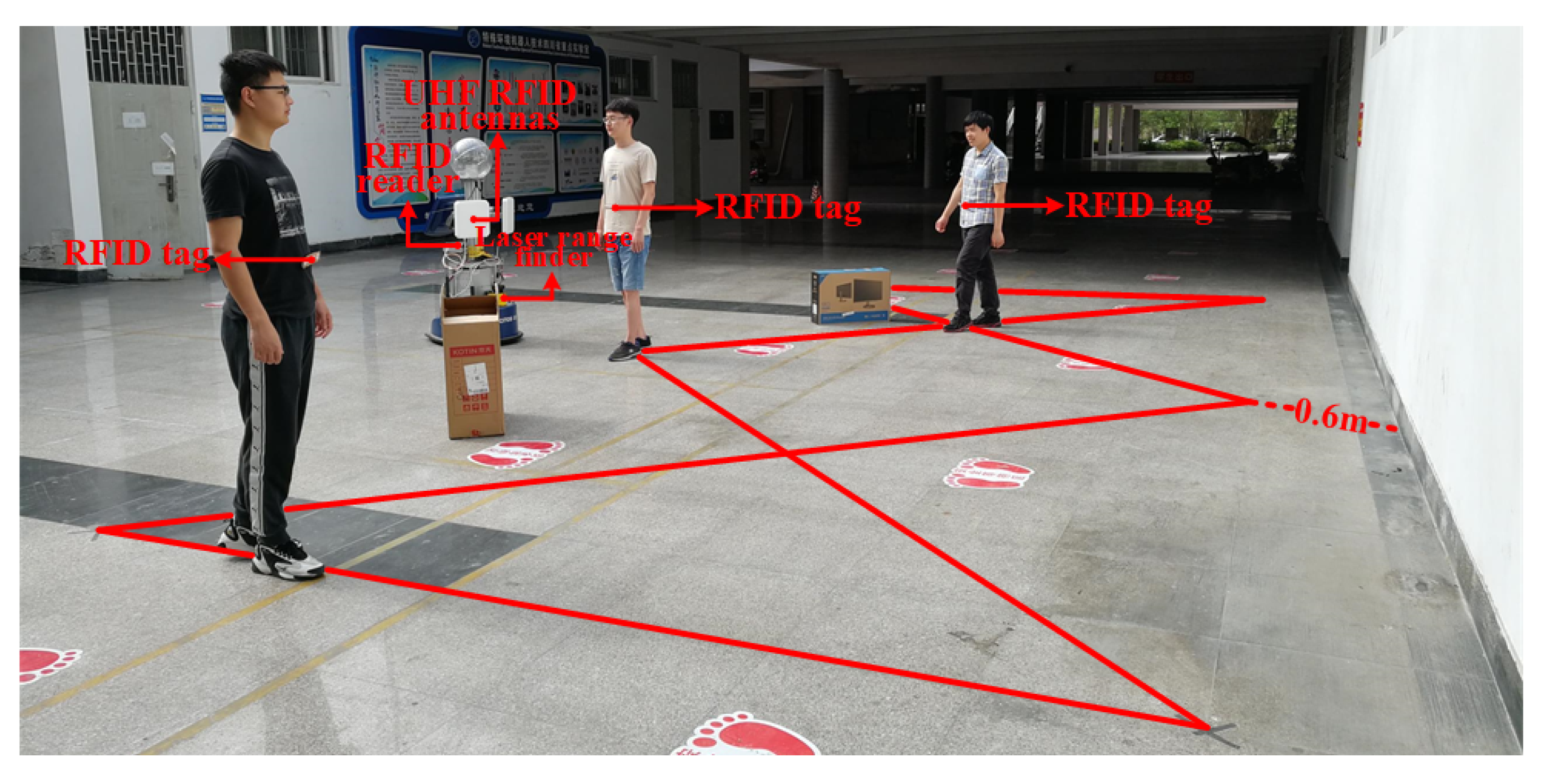
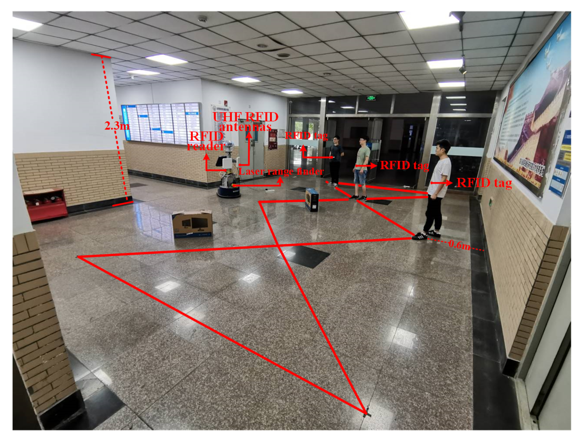
5.1. Experimental Setups
5.2. Impact of Different Methods on Experimental Results
5.3. Impact of Different Parameters on Experimental Results
5.3.1. The Influence of Antenna Settings on Experimental Results
5.3.2. The Influence of Phase Shift Threshold on Experimental Results
5.3.3. The Influence of The Number of Particles N on The Experimental Results
5.3.4. The Influence of The Time Window Size
5.4. Evaluation of the Approach with a Complex Path and a Different Environment
6. Conclusions
Author Contributions
Funding
Acknowledgments
Conflicts of Interest
Abbreviations
| UHF | Ultra High Frequency |
| BC | Bray-Curtis |
| RFID | Radio Frequency Identification |
| PF | Particle Filter |
| PCC | Pearson Correlation coefficent |
References
- Zafari, F.; Gkelias, A.; Leung, K.K. A survey of indoor localization systems and technologies. IEEE Commun. Surv. Tutor. 2019, 21, 2568–2599. [Google Scholar] [CrossRef] [Green Version]
- Luo, J.; Zhang, Z.; Liu, C.; Luo, H. Reliable and cooperative target tracking based on WSN and WiFi in indoor Wireless Networks. IEEE Access 2018, 6, 24846–24855. [Google Scholar] [CrossRef]
- Xu, D.; Han, L.; Tan, M.; Li, Y.F. Ceiling-based visual positioning for an indoor mobile robot with monocular vision. IEEE Trans. Ind. Electron. 2009, 56, 1617–1628. [Google Scholar]
- Wang, M.M.; Liu, Y.; Su, D.; Liao, Y.F.; Shi, L.; Xu, J.H.; Miro, J.V. Accurate and real-time 3-D tracking for the following robots by fusing vision and ultrasonar information. IEEE/ASME Trans. Mechatron. 2018, 23, 997–1006. [Google Scholar] [CrossRef]
- Liu, G.; Liu, S.; Muhammad, K.; Sangaiah, A.K.; Doctor, F. Object tracking in vary lighting conditions for fog based intelligent surveillance of public spaces. IEEE Access 2018, 6, 29283–29296. [Google Scholar] [CrossRef]
- Xing, B.Y.; Zhu, Q.M.; Pan, F.; Feng, X.X. Marker-based multi-sensor fusion indoor localization system for micro air vehicles. J. Sens. 2018, 18, 1706. [Google Scholar] [CrossRef] [PubMed] [Green Version]
- You, W.D.; Li, F.B.; Liao, L.Q.; Huang, M.L. Data fusion of UWB and IMU based on unscented Kalman filter for indoor localization of Quadrotor UAV. IEEE Access 2020, 8, 64971–64981. [Google Scholar] [CrossRef]
- Li, C.D.; Yu, L.; Fei, S.M. Real-Time 3D motion tracking and reconstruction system using camera and IMU sensors. IEEE Sens. J. 2019, 19, 6460–6466. [Google Scholar] [CrossRef]
- Peng, J.; Zhang, P.; Zheng, L.X.; Tan, J. UAV positioning based on multi-sensor fusion. IEEE Access 2020, 8, 34455–34467. [Google Scholar] [CrossRef]
- Shi, F.D.; Liu, W.H.; Wang, X.; Ding, J.; Shi, Y.J. Design of indoor lidar navigation system. Infrared Laser Eng. 2015, 44, 3570–3575. [Google Scholar]
- Zhao, X.M.; Sun, P.P.; Xu, Z.G.; Min, H.G.; Yu, H.K. Fusion of 3D LIDAR and camera data for object detection in autonomous vehicle applications. IEEE Sens. J. 2020, 20, 4901–4913. [Google Scholar] [CrossRef] [Green Version]
- DiGiampaolo, E.; Martinelli, F. Mobile robot localization using the phase of passive UHF RFID signals. IEEE Trans. Ind. Electron. 2014, 61, 365–376. [Google Scholar] [CrossRef]
- Tian, Q.L.; Wang, K.K.; Salcic, Z. A low-cost INS and UWB fusion pedestrian tracking system. IEEE Sens. J. 2019, 19, 3733–3740. [Google Scholar] [CrossRef]
- Wu, J.; Yu, Z.J.; Zhuge, J.C.; Xue, B. Indoor positioning by using scanning infrared laser and ultrasonic technology. Opt. Precis. Eng. 2016, 24, 2417–2423. [Google Scholar]
- Qu, H.K.; Zhang, Q.Y.; Ruan, Y.T. Laser radar based on scanning image tracking. Chin. Opt. 2012, 5, 242–247. [Google Scholar]
- Tang, J.; Chen, Y.W.; Jaakkola, A.; Liu, J.B.; Hyyppa, J.; Hyyppa, H. An UGV indoor positioning system using laser scan matching for large-area real-time applications. Sensors 2014, 14, 11805–11824. [Google Scholar] [CrossRef] [Green Version]
- Zhang, H.; Qiao, C.; Kuang, H.P. Object geo-location based on laser range finder for airborne electro-optical imaging systems. Opt. Precisioneng. 2019, 27, 8–16. [Google Scholar] [CrossRef]
- Liu, R.; Liang, G.L.; Wang, H.; Fu, Y.L.; He, J.; Zhang, H. Dynamic object location with radio frequency identification and laser information. J. Electron. Inf. 2018, 40, 55–62. [Google Scholar]
- Wang, D.Z.; Posner, I. Voting for voting in online point cloud object detection. Robot. Sci. Syst. 2015, 1, 1317. [Google Scholar]
- Huang, R.L.; Liang, H.W.; Chen, J.J.; Zhao, P.; Du, M.B. Detection, tracking and identification of dynamic obstacles in driverless vehicles based on laser radar. Robot 2016, 38, 437–443. [Google Scholar]
- Tong, X.Y.; Wu, R.; Yang, X.F.; Teng, S.H.; Zhuang, Y. Infrared and laser fusion object identification method. Infrared Laser Eng. 2018, 47, 167–174. [Google Scholar]
- Liu, R.; Husikć, G.; Zell, A. On Tracking dynamic objects with long range passive UHF RFID using a mobile robot. Int. J. Distrib. Sens. Netw. 2015, 11, 781380. [Google Scholar] [CrossRef]
- Fan, X.Y.; Wang, F.; Gong, W.; Zhang, L.; Liu, J.C. Multiple object activity identification using RFIDs: A multipath-aware deep learning solution. In Proceedings of the 2018 IEEE 38th International Conference on Distributed Computing Systems (ICDCS), Vienna, Austria, 2–6 July 2018; pp. 545–555. [Google Scholar]
- Ni, L.M.; Liu, Y.H.; Lau, Y.C.; Patil, A.P. LANDMARC: Indoor location sensing using active RFID. Wirel. Netw. 2004, 10, 701–710. [Google Scholar] [CrossRef]
- Hightower, J.; Borriello, G.; Wang, R. SpotON: An Indoor 3D Location Sensing Technology Based on RF Signal Strength; Technic Report 2000-02-02; Department of Computer Science and Engineering, University of Washington: Seattle, WA, USA, 2000. [Google Scholar]
- Zhao, Y.Y.; Liu, Y.H.; Ni, L.M. VIRE: Active RFID-based localization using Virtual Reference Elimination. In Proceedings of the 2007 International Conference on Parallel Processing (ICPP 2007), Xi’an, China, 10–14 September 2007; p. 56. [Google Scholar]
- Alvarado Vasquez, B.P.E.; Gonzalez, R.; Matia, F.; De La Puente, P. Sensor fusion for tour-guide robot localization. IEEE Access 2018, 6, 78947–78964. [Google Scholar] [CrossRef]
- Choi, B.S.; Lee, J.W.; Park, K.T. A hierarchical algorithm for indoor mobile robot localization using rfid sensor fusion. IEEE Trans. Ind. Electron. 2011, 58, 2226–2235. [Google Scholar] [CrossRef]
- Suparyanto, A.; Fatimah, R.N.; Widyotriatmo, A.; Nazaruddin, Y.Y. Port container truck localization using sensor fusion technique. In Proceedings of the 2018 5th International Conference on Electric Vehicular Technology (ICEVT), Surakarta, Indonesia, 30–31 October 2018; pp. 72–77. [Google Scholar]
- Wang, C.S.; Chen, C.L. RFID-based and Kinect-based indoor positioning system. In Proceedings of the 2014 4th International Conference on Wireless Communications, Vehicular Technology, Information Theory and Aerospace & Electronic Systems (VITAE), Aalborg, Denmark, 11–14 May 2014; pp. 1–4. [Google Scholar]
- Li, X.Y.; Zhang, Y.Z.; Marsic, I.; Burd, R.S. Online people tracking and identification with RFID and Kinect. arXiv 2017, arXiv:1702.03824. [Google Scholar]
- Parr, A.; Miesen, R.; Kirsch, F.; Vossiek, M. A novel method for UHF RFID tag tracking based on acceleration data. In Proceedings of the 2012 IEEE International Conference on RFID (RFID), Orlando, FL, USA, 3–5 April 2012; pp. 110–115. [Google Scholar]
- Faramondi, L.; Inderst, F.; Pascucci, F.; Setola, R.; Delprato, U. An enhanced indoor positioning system for first responders. In Proceedings of the International Conference on Indoor Positioning and Indoor Navigation, Montbeliard-Belfort, France, 28–31 October 2013; pp. 1–8. [Google Scholar]
- Vorst, P.; Zell, A. A comparison of similarity measures for localization with passive rfid fingerprints. In Proceedings of the ISR 2010 (41st International Symposium on Robotics) and ROBOTIK 2010 (6th German Conference on Robotics), Munich, Germany, 7–9 June 2010; pp. 1–8. [Google Scholar]
- Vorst, P.; Koch, A.; Zell, A. Efficient self-adjusting, similarity-based location fingerprinting with passive UHF RFID. In Proceedings of the 2011 IEEE International Conference on RFID-Technologies and Applications, Sitges, Spain, 15–16 September 2011; pp. 160–167. [Google Scholar]
- Shyam, R.; Singh, Y.N. Face recognition using augmented local binary pattern and Bray Curtis dissimilarity metric. In Proceedings of the 2015 2nd International Conference on Signal Processing and Integrated Networks (SPIN), Noida, India, 19–20 February 2015; pp. 779–784. [Google Scholar]
- Samantaray, A.K.; Rahulkar, A.D. Comparison of similarity measurement metrics on medical image data. In Proceedings of the 2019 10th International Conference on Computing, Communication and Networking Technologies (ICCCNT), Kanpur, India, 6–8 July 2019; pp. 1–5. [Google Scholar]
- Li, X.; Zhang, Y.; Amin, M.G. Multifrequency-based range estimation of RFID Tags. In Proceedings of the 2009 IEEE International Conference on RFID, Orlando, FL, USA, 27–28 April 2009; pp. 147–154. [Google Scholar]
- Li, S.S. An improved DBSCAN algorithm based on the neighbor similarity and fast nearest neighbor query. IEEE Access 2020, 8, 47468–47476. [Google Scholar] [CrossRef]
- Fu, Y.L.; Liu, R.; Zhang, H.; Liang, G.L.; Shafiq, U.R.; Liu, L.X. Continuously tracking of moving object by a combination of ultra-high frequency radio-frequency identification and laser range finder. Int. J. Distrib. Sens. Netw. 2019, 7. [Google Scholar] [CrossRef] [Green Version]
- Zhu, H.; You, X.; Liu, S. Multiple ant colony optimization based on Pearson Correlation Coefficient. IEEE Access 2019, 7, 61628–61638. [Google Scholar] [CrossRef]
- Chen, G.; Liu, Q.; Wei, Y.K.; Yu, Q. An efficient indoor location system in WLAN based on database partition and euclidean distance-weighted Pearson Correlation Coefficient. In Proceedings of the 2016 2nd IEEE International Conference on Computer and Communications (ICCC), Chengdu, China, 14–17 October 2016; pp. 1736–1741. [Google Scholar]
- Cardoso, A.D.V.; Nedjah, N.; Macedo Mourelle, L.D. Accelerating template matching for efficient object tracking. In Proceedings of the 2019 IEEE 10th Latin American Symposium on Circuits & Systems (LASCAS), Armenia, Colombia, 24–27 February 2019; pp. 141–144. [Google Scholar]


| Mathematical Symbol | Meaning |
|---|---|
| The similarity between phase-based radial velocity and laser cluster-based radial velocity | |
| w | The size of each time window |
| RFID phase-based radial velocity at time t | |
| Radial velocity of the i-th cluster at time t | |
| The phase of RFID signal at time t | |
| The radial distance from the moving tag to the antenna at time t | |
| Phase difference | |
| The phase differences after normalized to the main value interval of | |
| Clusters in total at time t | |
| Center coordinates of the j-th cluster at time t | |
| The radial velocity of cluster i at time t | |
| N | Number of particles |
| The position of particle n to track i-th cluster at time t | |
| The weight of particle n to track i-th cluster at time t | |
| The Gaussian noise with zero mean and standed deviation of | |
| The normalization coefficient |
| Methods | Localization Error (m) | Matching Rate (%) |
|---|---|---|
| BC | 0.76 | 79.2 |
| PF + BC | 0.65 | 83.1 |
| PCC + PF + BC | 0.33 | 90.2 |
| Antenna Combination | Methods | Localization Error (m) |
|---|---|---|
| BC | 0.88 | |
| Only Right Antenna | PF + BC | 0.96 |
| PCC + PF + BC | 0.82 | |
| BC | 0.68 | |
| Only Left Antenna | PF + BC | 0.89 |
| PCC + PF + BC | 0.61 | |
| BC | 0.76 | |
| Both | PF + BC | 0.65 |
| PCC + PF + BC | 0.33 |
| Methods | Localization Error (m) | Matching Rate (%) | |
|---|---|---|---|
| BC | 2.41 | 54.9 | |
| PF + BC | 1.98 | 64.0 | |
| PCC + PF + BC | 0.72 | 81.6 | |
| BC | 0.88 | 66.4 | |
| PF + BC | 0.72 | 82.1 | |
| PCC + PF + BC | 0.34 | 88.2 | |
| BC | 0.79 | 68.1 | |
| PF + BC | 0.63 | 85.2 | |
| PCC + PF + BC | 0.36 | 87.6 | |
| BC | 0.76 | 79.2 | |
| PF + BC | 0.65 | 83.1 | |
| PCC + PF + BC | 0.33 | 90.2 | |
| BC | 0.76 | 78.8 | |
| PF + BC | 0.68 | 81.4 | |
| PCC + PF + BC | 0.37 | 84.2 | |
| BC | 0.77 | 78.9 | |
| PF + BC | 0.67 | 81.8 | |
| PCC + PF + BC | 0.38 | 83.8 | |
| BC | 0.86 | 66.7 | |
| PF + BC | 0.81 | 67.1 | |
| PCC + PF + BC | 0.83 | 66.8 |
| Number of Particles N | Localization Error (m) | Time Consumption (ms) |
|---|---|---|
| 5 | 1.41 | 2.96 |
| 20 | 0.44 | 3.99 |
| 50 | 0.37 | 5.16 |
| 100 | 0.35 | 5.82 |
| 200 | 0.33 | 6.44 |
| 400 | 0.32 | 8.30 |
| 1000 | 0.33 | 12.17 |
| Window Size w (s) | Method | The Average Distance Traveled in Each Window (m) | Localization Error (m) | Matching Rate (%) | Time Consumption (ms) |
|---|---|---|---|---|---|
| 5 | BC | 0.93 | 1.14 | 66.9 | 28.16 |
| PF + BC | 0.93 | 0.88 | 72.5 | 34.42 | |
| PCC + PF + BC | 0.93 | 0.71 | 81.8 | 42.56 | |
| 15 | BC | 2.79 | 0.86 | 67.2 | 30.3 |
| PF + BC | 2.79 | 0.67 | 82.8 | 38.36 | |
| PCC + PF + BC | 2.79 | 0.37 | 87.0 | 46.42 | |
| 25 | BC | 4.65 | 0.76 | 79.2 | 33.28 |
| PF + BC | 4.65 | 0.65 | 83.1 | 43.1 | |
| PCC + PF + BC | 4.65 | 0.33 | 90.2 | 51.07 | |
| 35 | BC | 6.51 | 0.81 | 68.3 | 34.69 |
| PF + BC | 6.51 | 0.70 | 82.3 | 46.97 | |
| PCC + PF + BC | 6.51 | 0.33 | 87.7 | 54.81 | |
| 50 | BC | 9.18 | 0.83 | 67.6 | 38.41 |
| PF + BC | 9.18 | 0.64 | 83.8 | 54.69 | |
| PCC + PF + BC | 9.18 | 0.35 | 87.6 | 62.24 |
| Methods | Localization Error (m) |
|---|---|
| BC | 0.82 |
| PF + BC | 0.68 |
| PCC + PF + BC | 0.44 |
© 2020 by the authors. Licensee MDPI, Basel, Switzerland. This article is an open access article distributed under the terms and conditions of the Creative Commons Attribution (CC BY) license (http://creativecommons.org/licenses/by/4.0/).
Share and Cite
Fu, W.; Liu, R.; Wang, H.; Ali, R.; He, Y.; Cao, Z.; Qin, Z. A Method of Multiple Dynamic Objects Identification and Localization Based on Laser and RFID. Sensors 2020, 20, 3948. https://doi.org/10.3390/s20143948
Fu W, Liu R, Wang H, Ali R, He Y, Cao Z, Qin Z. A Method of Multiple Dynamic Objects Identification and Localization Based on Laser and RFID. Sensors. 2020; 20(14):3948. https://doi.org/10.3390/s20143948
Chicago/Turabian StyleFu, Wenpeng, Ran Liu, Heng Wang, Rashid Ali, Yongping He, Zhiqiang Cao, and Zhenghong Qin. 2020. "A Method of Multiple Dynamic Objects Identification and Localization Based on Laser and RFID" Sensors 20, no. 14: 3948. https://doi.org/10.3390/s20143948