Accurate Spirometry with Integrated Barometric Sensors in Face-Worn Garments


Abstract
1. Introduction
1.1. Novelty and Contribution
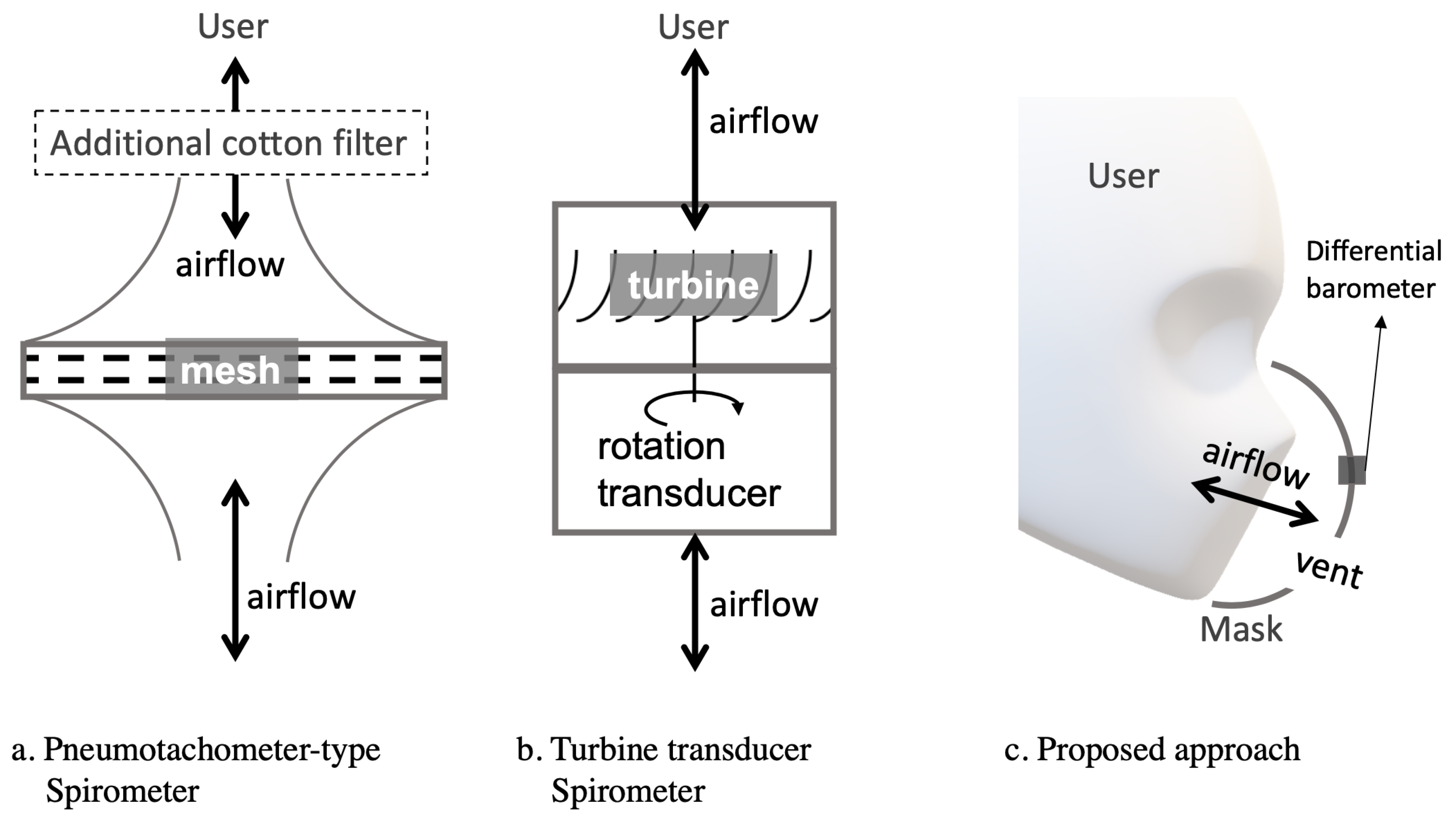
- We demonstrate the possibility of performing accurate transient breathing volume measurement in a wearable garment in the form of a sports mask, as opposed to hand-held novel spirometers, which mostly require a specific structure with a breathing tube, as reviewed in Section 2.2.
- Our approach uses only off-the-shelf components, without any proprietary sensors or custom mechanical designs.
- The only sensing element needed is a pair of low-cost (three Euros) miniaturized (2.5 millimeters) barometric pressure sensors that are already widely available thanks to the personal mobile devices and drone industry.
- The approach is made possible by shifting the measurement modality, from directly placing sensors in the airflow duct to elaborating the pressure difference of the inside and outside of the face mask compartment, as shown in Figure 1.
1.2. Paper Structure
2. Background and State-of-the-Art
2.1. Pulmonary Function Tests
2.2. Spirometry Devices
2.3. Respiration Monitoring in Wearable and Pervasive Research
3. Hardware
3.1. Embedded Barometer and Electronics Hardware
3.2. Mask-to-Spirometer Calibration Setup
3.3. Spirometer-to-Spirometer Reference
4. Understanding Airflow and Pressure
5. Forced Vital Capacity Test
Experiment Procedure
6. Signal Processing
6.1. Physical Model Fitting
6.2. Polynomial Curve Fitting
6.3. Neural Network Regression
6.4. Participant Pool Division Schemes
- Individual: A separate model was fitted with the data samples from every participant.
- Inclusive: A single model was fitted with the data sampled from all participants combined.
- Exclusive: The 20 participants were randomly divided into five folds. A separate model was fitted with data from four folds and tested on the remaining fold.
7. Results and Discussion
7.1. Predict FVC with Barometers
7.2. Person Dependency and Customized Fitting
7.3. Continuous Tidal Volume Monitoring
7.4. The Newer Barometer Version
- operation range of 300 to 1250 hPa over 300 to 1100 hPa,
- barometer noise of 0.03 Pa over 0.2Pa,
- temperature coefficient offset 0.75 Pa/K over 1.5 Pa/K,
- relative accuracy of 8 Pa over 12 Pa,
- output resolution 0.016 Pa over 0.18 Pa,
- one year stability 0.33 hPa over 1 hPa,
- retail price of two Euros over three Euros (as BMP388 lacks the humidity sensor component).
7.5. Performance and Wearable Prospect
- Conditioning the sensor’s raw data through subtraction, removing offset, and filtering, resulting in the differential pressure value.
- Predicting the air flow from the pressure value using the regression model.
- Generating results of the pulmonary function test parameters from the flow-volume loop.
8. Conclusions
8.1. Summary
8.2. Wearable Outlook
Author Contributions
Funding
Conflicts of Interest
References
- Technavio. Global Sports and Fitness Wear Market 2019–2023. Available online: www.businesswire.com/news/home/20191126005547/en/Global-Sports-Fitness-Wear-Market-2019-2023-Evolving (accessed on 26 July 2020).
- Conkle, J.P.; Camp, B.J.; Welch, B.E. Trace composition of human respiratory gas. Arch. Environ. Health Int. J. 1975, 30, 290–295. [Google Scholar] [CrossRef] [PubMed]
- Whipp, B.J.; Ward, S.A.; Lamarra, N.; Davis, J.A.; Wasserman, K. Parameters of ventilatory and gas exchange dynamics during exercise. J. Appl. Physiol. 1982, 52, 1506–1513. [Google Scholar] [PubMed]
- Kory, R.C.; Callahan, R.; Boren, H.G.; Syner, J.C. The Veterans Administration-Army cooperative study of pulmonary function: I. Clinical spirometry in normal men. Am. J. Med. 1961, 30, 243–258. [Google Scholar] [CrossRef]
- Stock, M.C.; Downs, J.B.; Gauer, P.K.; Alster, J.M.; Imrey, P.B. Prevention of postoperative pulmonary complications with CPAP, incentive spirometry, and conservative therapy. Chest 1985, 87, 151–157. [Google Scholar] [CrossRef]
- Kispert, J.; Kazmers, A.; Roitman, L. Preoperative spirometry predicts perioperative pulmonary complications after major vascular surgery. Am. Surg. 1992, 58, 491–495. [Google Scholar]
- Sherratt, R.S.; Dey, N. Low-Power Wearable Healthcare Sensors. Electronics 2020, 9, 892. [Google Scholar] [CrossRef]
- Hull, J.H.; Lloyd, J.K.; Cooper, B.G. Lung function testing in the COVID-19 endemic. Lancet Respir. Med. 2020, 8, 666–667. [Google Scholar] [CrossRef]
- Lee, K.H.; Hui, K.P.; Chan, T.B.; Tan, W.C.; Lim, T.K. Rapid shallow breathing (frequency-tidal volume ratio) did not predict extubation outcome. Chest 1994, 105, 540–543. [Google Scholar] [CrossRef]
- Vassilakopoulos, T.; Zakynthinos, S.; Roussos, C. The tension–time index and the frequency/tidal volume ratio are the major pathophysiologic determinants of weaning failure and success. Am. J. Respir. Crit. Care Med. 1998, 158, 378–385. [Google Scholar] [CrossRef] [PubMed]
- Hey, E.; Lloyd, B.; Cunningham, D.; Jukes, M.; Bolton, D. Effects of various respiratory stimuli on the depth and frequency of breathing in man. Respir. Physiol. 1966, 1, 193–205. [Google Scholar] [CrossRef]
- Cotes, J.; Johnson, G.; Mcdonald, A. Breathing frequency and tidal volume: Relationship to breathlessness. In Breathing: Hering-Breuer Centenary Symposium; Churchill: London, UK, 1970; pp. 297–314. [Google Scholar] [CrossRef]
- Miller, M.R.; Hankinson, J.; Brusasco, V.; Burgos, F.; Casaburi, R.; Coates, A.; Crapo, R.; Enright, P.V.; Van Der Grinten, C.; Gustafsson, P.; et al. Standardisation of spirometry. Eur. Respir. J. 2005, 26, 319–338. [Google Scholar] [CrossRef] [PubMed]
- Emmanuel, G.; Briscoe, W.; Cournand, A. A method for the determination of the volume of air in the lungs: Measurements in chronic pulmonary emphysema. J. Clin. Investig. 1961, 40, 329–337. [Google Scholar] [PubMed]
- McCartney, C.T.; Weis, M.N.; Ruppel, G.L.; Nayak, R.P. Residual volume and total lung capacity to assess reversibility in obstructive lung disease. Respir. Care 2016, 61, 1505–1512. [Google Scholar] [CrossRef] [PubMed]
- Choi, J.Y.; Rha, D.w.; Park, E.S. Change in pulmonary function after incentive spirometer exercise in children with spastic cerebral palsy: A randomized controlled study. Yonsei Med. J. 2016, 57, 769–775. [Google Scholar] [CrossRef] [PubMed]
- Eltorai, A.E.; Baird, G.L.; Eltorai, A.S.; Healey, T.T.; Agarwal, S.; Ventetuolo, C.E.; Martin, T.J.; Chen, J.; Kazemi, L.; Keable, C.A.; et al. Effect of an incentive spirometer patient reminder after coronary artery bypass grafting: A randomized clinical trial. JAMA Surg. 2019, 154, 579–588. [Google Scholar] [CrossRef] [PubMed]
- Sokol, Y.; Tomashevsky, R.; Kolisnyk, K. Turbine spirometers metrological support. In Proceedings of the 2016 International Conference on Electronics and Information Technology (EIT), Odessa, Ukraine, 23–27 May 2016; pp. 1–4. [Google Scholar]
- Wohlgemuth, M.; Van der Kooi, E.; Hendriks, J.; Padberg, G.; Folgering, H. Face mask spirometry and respiratory pressures in normal subjects. Eur. Respir. J. 2003, 22, 1001–1006. [Google Scholar] [CrossRef]
- Abdelgawad, T.T.; Abumossalam, A.M.; Abdalla, D.A.; Elsayed, M.E.M. Spirometry using face mask versus conventional tube in patients with neuromuscular disorders. Egypt. J. Chest Dis. Tuberc. 2017, 66, 717–722. [Google Scholar] [CrossRef]
- Rothe, T.; Karrer, W.; Schindler, C. Accuracy of the piko-1 pocket spirometer. J. Asthma 2012, 49, 45–50. [Google Scholar]
- McCarthy, K. Selecting Spirometers for Home Testing. Respir. Ther. 2017, 12, 14–17. [Google Scholar]
- AL-Khalidi, F.Q.; Saatchi, R.; Burke, D.; Elphick, H.; Tan, S. Respiration rate monitoring methods: A review. Pediatr. Pulmonol. 2011, 46, 523–529. [Google Scholar] [CrossRef]
- Sakka, E.J.; Aggelidis, P.; Psimarnou, M. Mobispiro: A novel spirometer. In XII Mediterranean Conference on Medical and Biological Engineering and Computing; Springer: Berlin/Heidelberg, Germany, 2010; pp. 498–501. [Google Scholar]
- Xu, X.K.; Harvey, B.P.; Lutchen, K.R.; Gelbman, B.D.; Monfre, S.L.; Coifman, R.E.; Forbes, C.E. Comparison of a micro-electro-mechanical system airflow sensor with the pneumotach in the forced oscillation technique. Med. Dev. 2018, 11, 419. [Google Scholar] [CrossRef] [PubMed]
- Ambastha, S.; Umesh, S.; Maheshwari, U.; Asokan, S. Pulmonary function test using fiber Bragg grating spirometer. J. Lightwave Technol. 2016, 34, 5682–5688. [Google Scholar] [CrossRef]
- Fung, A.G.; Tan, L.D.; Duong, T.N.; Schivo, M.; Littlefield, L.; Delplanque, J.P.; Davis, C.E.; Kenyon, N.J. Design and Benchmark Testing for Open Architecture Reconfigurable Mobile Spirometer and Exhaled Breath Monitor with GPS and Data Telemetry. Diagnostics 2019, 9, 100. [Google Scholar] [CrossRef] [PubMed]
- Zhou, P.; Yang, L.; Huang, Y.X. A smart phone based handheld wireless spirometer with functions and precision comparable to laboratory spirometers. Sensors 2019, 19, 2487. [Google Scholar] [CrossRef]
- Chee, Y.; Han, J.; Youn, J.; Park, K. Air mattress sensor system with balancing tube for unconstrained measurement of respiration and heart beat movements. Physiol. Meas. 2005, 26, 413. [Google Scholar] [CrossRef] [PubMed]
- Watanabe, K.; Watanabe, T.; Watanabe, H.; Ando, H.; Ishikawa, T.; Kobayashi, K. Noninvasive measurement of heartbeat, respiration, snoring and body movements of a subject in bed via a pneumatic method. IEEE Trans. Biomed. Eng. 2005, 52, 2100–2107. [Google Scholar] [CrossRef] [PubMed]
- Ho, K.; Tsuchiya, N.; Nakajima, H.; Kuramoto, K.; Kobashi, S.; Hata, Y. Fuzzy logic approach to respiration detection by air pressure sensor. In Proceedings of the IEEE International Conference on Fuzzy Systems, Jeju Island, Korea, 20–24 August 2009; pp. 911–915. [Google Scholar]
- Kundu, S.K.; Kumagai, S.; Sasaki, M. A wearable capacitive sensor for monitoring human respiratory rate. Jpn. J. Appl. Phys. 2013, 52, 04CL05. [Google Scholar] [CrossRef]
- Cheng, J.; Amft, O.; Lukowicz, P. Active capacitive sensing: Exploring a new wearable sensing modality for activity recognition. In International Conference on Pervasive Computing; Springer: Berlin/Heidelberg, Germany, 2010; pp. 319–336. [Google Scholar]
- Konno, K.; Mead, J. Measurement of the separate volume changes of rib cage and abdomen during breathing. J. Appl. Physiol. 1967, 22, 407–422. [Google Scholar]
- Guo, L.; Berglin, L.; Li, Y.; Mattila, H.; Mehrjerdi, A.K.; Skrifvars, M. ’Disappearing Sensor’-Textile Based Sensor for Monitoring Breathing. In Proceedings of the International Conference on Control, Automation and Systems Engineering (CASE), Singapore, 30–31 July 2011; pp. 1–4. [Google Scholar]
- Guo, L.; Peterson, J.; Qureshi, W.; Kalantar Mehrjerdi, A.; Skrifvars, M.; Berglin, L. Knitted Wearable Stretch Sensor for Breathing Monitoring Application. In Proceedings of the Ambience’11, Borås, Sweden, 28–30 November 2011; Available online: www.diva-portal.org/smash/get/diva2:887398/FULLTEXT01.pdf (accessed on 26 July 2020).
- Yang, X.; Chen, Z.; Elvin, C.S.M.; Janice, L.H.Y.; Ng, S.H.; Teo, J.T.; Wu, R. Textile fiber optic microbend sensor used for heartbeat and respiration monitoring. IEEE Sens. J. 2014, 15, 757–761. [Google Scholar] [CrossRef]
- Servati, A.; Zou, L.; Wang, Z.J.; Ko, F.; Servati, P. Novel flexible wearable sensor materials and signal processing for vital sign and human activity monitoring. Sensors 2017, 17, 1622. [Google Scholar] [CrossRef]
- Al-Halhouli, A.; Al-Ghussain, L.; El Bouri, S.; Liu, H.; Zheng, D. Fabrication and evaluation of a novel non-invasive stretchable and wearable respiratory rate sensor based on silver nanoparticles using inkjet printing technology. Polymers 2019, 11, 1518. [Google Scholar] [CrossRef]
- Jackson, C.; Lees, H. The correlations between vital capacity and various physical measurements in one hundred healthy male university students. Am. J. Physiol.-Legacy Content 1929, 87, 654–666. [Google Scholar] [CrossRef][Green Version]
- Oletic, D.; Arsenali, B.; Bilas, V. Low-power wearable respiratory sound sensing. Sensors 2014, 14, 6535–6566. [Google Scholar] [CrossRef] [PubMed]
- Liu, G.; Iwai, M.; Tobe, Y.; Matekenya, D.; Hossain, K.M.A.; Ito, M.; Sezaki, K. Beyond horizontal location context: Measuring elevation using smartphone’s barometer. In Proceedings of the 2014 ACM International Joint Conference on Pervasive and Ubiquitous Computing: Adjunct Publication, Seattle, WA, USA, 13–17 September 2014; pp. 459–468. [Google Scholar]
- Li, Y.; Zahran, S.; Zhuang, Y.; Gao, Z.; Luo, Y.; He, Z.; Pei, L.; Chen, R.; El-Sheimy, N. IMU/magnetometer/barometer/mass-flow sensor integrated indoor quadrotor UAV localization with robust velocity updates. Remote Sens. 2019, 11, 838. [Google Scholar] [CrossRef]
- Ao, J.; Wu, X.; Wang, T.; Feng, Z.; Sungki, L. UAV Having Barometric Sensor and Method of Isolating Disposing Barometric Sensor within UAV. U.S. Patent 10,611,476, 8 December 2016. [Google Scholar]
- Costa, A.B.; Zhou, B.; Amiraslanov, O.; Lukowicz, P. Wearable Spirometry: Using Integrated Environment Sensor for Breath Measurement. In NexTech 2018, International Conference on Mobile Ubiquitous Computing, Systems, Services and Technologies (UBICOMM-2018), Athens, Greece, 18–22 November 2018; IARIA XPS Press: Redhook, NY, USA, 2018; ISBN 978-1-61208-676-7. [Google Scholar]
- Zhou, B.; Costa, A.B.; Lukowicz, P. CoRSA: A cardio-respiratory monitor in sport activities. In Proceedings of the 23rd International Symposium on Wearable Computers, London, UK, 9–13 September 2019; pp. 254–256. [Google Scholar]
- Patrick, J.; Howard, A. The influence of age, sex, body size and lung size on the control and pattern of breathing during CO2 inhalation in Caucasians. Respir. Physiol. 1972, 16, 337–350. [Google Scholar] [CrossRef]
- Hart, M.C.; Orzalesi, M.M.; Cook, C.D. Relation between anatomic respiratory dead space and body size and lung volume. J. Appl. Physiol. 1963, 18, 519–522. [Google Scholar] [CrossRef]
- Kähler, C.J.; Hain, R. Flow Analyses to Validate SARS-CoV-2 Protective Masks. 2020. Available online: www.unibw.de/lrt7-en/flow-analyses-to-validate-sars-cov-2-protective-masks (accessed on 26 July 2020).
- Johnson, A.T.; Cummings, E.G. Mask design considerations. Am. Ind. Hyg. Assoc. J. 1975, 36, 220–228. [Google Scholar] [CrossRef]
- Smith, K. On the standard deviations of adjusted and interpolated values of an observed polynomial function and its constants and the guidance they give towards a proper choice of the distribution of observations. Biometrika 1918, 12, 1–85. [Google Scholar] [CrossRef]
- Levenberg, K. A method for the solution of certain non-linear problems in least squares. Q. Appl. Math. 1944, 2, 164–168. [Google Scholar] [CrossRef]
- Marquardt, D.W. An algorithm for least-squares estimation of nonlinear parameters. J. Soc. Ind. Appl. Math. 1963, 11, 431–441. [Google Scholar] [CrossRef]
- Jensen, R.L.; Teeter, J.G.; England, R.D.; White, H.J.; Pickering, E.H.; Crapo, R.O. Instrument accuracy and reproducibility in measurements of pulmonary function. Chest 2007, 132, 388–395. [Google Scholar] [CrossRef] [PubMed]
Sample Availability: Data and source code of this study are available from the authors. |


| Model | a | b | c | d | e |
|---|---|---|---|---|---|
| root2only | - | - | 0.1744 | - | - |
| - | - | −0.1373 | - | - | |
| root2 | 0.0049 | −0.3337 | 0.1466 | - | - |
| −0.0043 | 0.1956 | −0.1150 | - | - | |
| root3 | 0.0001 | 0.3187 | 0.5472 | −0.8883 | - |
| −0.0008 | −0.1054 | −0.3421 | 0.4707 | - | |
| root4 | −0.0020 | −0.0045 | 0.9210 | −3.0140 | 2.1070 |
| 0.0007 | 0.0085 | −0.5331 | 1.4570 | −0.9274 |
| Model | ||||||
|---|---|---|---|---|---|---|
| poly2 | 0.7420 | 1.5460 | −0.0768 | - | - | - |
| poly3 | 0.7747 | 1.6290 | −0.1562 | 0.0073 | - | - |
| poly4 | 0.7892 | 1.6550 | −0.2128 | 0.0194 | −0.0063 | - |
| poly5 | −0.0487 | 0.0207 | −0.0001 | 0.0000 | 0.0000 | 0.0000 |
| Root | RMSE | Polynomial | RMSE | Neural Network | RMSE |
|---|---|---|---|---|---|
| root2only | 0.4237 | Poly2 | 0.2152 | ANN1 | 0.2371 |
| root2 | 0.2085 | Poly3 | 0.1989 | ANN3 | 0.2243 |
| root3 | 0.1939 | Poly4 | 0.1934 | ANN5 | 0.1955 |
| root4 | 0.1926 | Poly5 | 0.1921 | ANN7 | 0.1954 |
| FVC Vitals | Tidal Breathing | ||||||
|---|---|---|---|---|---|---|---|
| FEV1 | FVC | PEF | FEF25 | FIF25 | Airflow | Volume (TV) | |
| Exclusive (root4) | 0.0591 | 0.0562 | 0.0406 | 0.0423 | 0.0372 | 0.0296 | 0.0285 |
| Inclusive (root4) | 0.0587 | 0.0553 | 0.0388 | 0.0410 | 0.0349 | 0.0249 | 0.0232 |
| Individual (root4) | 0.0318 | 0.0321 | 0.0241 | 0.0272 | 0.0219 | 0.0196 | 0.0159 |
| Exclusive (poly5) | 0.0600 | 0.0521 | 0.0411 | 0.0452 | 0.0335 | 0.0362 | 0.0439 |
| Inclusive (poly5) | 0.0600 | 0.0514 | 0.0378 | 0.0427 | 0.0309 | 0.0246 | 0.0227 |
| Individual (poly5) | 0.0303 | 0.0381 | 0.0270 | 0.0274 | 0.0203 | 0.0194 | 0.0154 |
| Exclusive (ANN7) | 0.0587 | 0.0518 | 0.0396 | 0.0423 | 0.0362 | 0.0251 | 0.0232 |
| Inclusive (ANN7) | 0.0577 | 0.0510 | 0.0369 | 0.0398 | 0.0316 | 0.0243 | 0.0225 |
| Individual (ANN7) | 0.0286 | 0.0327 | 0.0248 | 0.0232 | 0.0224 | 0.0192 | 0.0150 |
| Model | Conditioning | Predicting | Generating Results | Total Online | Offline Training |
|---|---|---|---|---|---|
| root4 | 0.0001 | 0.0967 | 0.0001 | 0.0969 | 0.7681 |
| poly5 | 0.0001 | 0.0270 | 0.0001 | 0.0272 | 0.0762 |
| ANN7 | 0.0001 | 0.0003 | 0.0001 | 0.0005 | 0.0300 |
| Study | Description | FVC | PEF | FEV1 | TV | Flow Range |
|---|---|---|---|---|---|---|
| Our Approach | BME280 pair | 3.3% | 2.5% | 2.9% | 1.5% | −7∼12 L/s |
| MobiSpiro [24] | custom MEMS | 3% | 5% | 3% | 5% | 0∼14 L/s |
| FBG [26] | optical fiber | 20% | 8% | 24% | - | 2∼8 L/s |
| Open Spirometer [27] | piezoresistive pressure sensors | 6% | - | 2% | - | 0∼15 L/s |
| Mobile Spirometer [28] | pneumotachometer | - | - | - | - | 0∼15 L/s |
| ATS/ERS [13,54] | medical society requirement | 3% | 10% | 3% | 3% | 0∼14 L/s |
- 1:
- This is the range of our participants’ data. Obviously, a person’s inhale peak flow is less powerful than exhale. However, the barometer’s operation range is at least 100 times more than the range we observed in our experiment.
- 2:
- The study in [27] used correlation R as the evaluation measure, and we converted it with 1-R to compare with others.
- 3:
- Pulmonary function tests were not performed in the evaluation [28].
© 2020 by the authors. Licensee MDPI, Basel, Switzerland. This article is an open access article distributed under the terms and conditions of the Creative Commons Attribution (CC BY) license (http://creativecommons.org/licenses/by/4.0/).
Share and Cite
Zhou, B.; Baucells Costa, A.; Lukowicz, P. Accurate Spirometry with Integrated Barometric Sensors in Face-Worn Garments. Sensors 2020, 20, 4234. https://doi.org/10.3390/s20154234
Zhou B, Baucells Costa A, Lukowicz P. Accurate Spirometry with Integrated Barometric Sensors in Face-Worn Garments. Sensors. 2020; 20(15):4234. https://doi.org/10.3390/s20154234
Chicago/Turabian StyleZhou, Bo, Alejandro Baucells Costa, and Paul Lukowicz. 2020. "Accurate Spirometry with Integrated Barometric Sensors in Face-Worn Garments" Sensors 20, no. 15: 4234. https://doi.org/10.3390/s20154234
APA StyleZhou, B., Baucells Costa, A., & Lukowicz, P. (2020). Accurate Spirometry with Integrated Barometric Sensors in Face-Worn Garments. Sensors, 20(15), 4234. https://doi.org/10.3390/s20154234