In-Service Detection and Quantification of Railway Wheel Flat by the Reflective Optical Position Sensor


Abstract
:1. Introduction
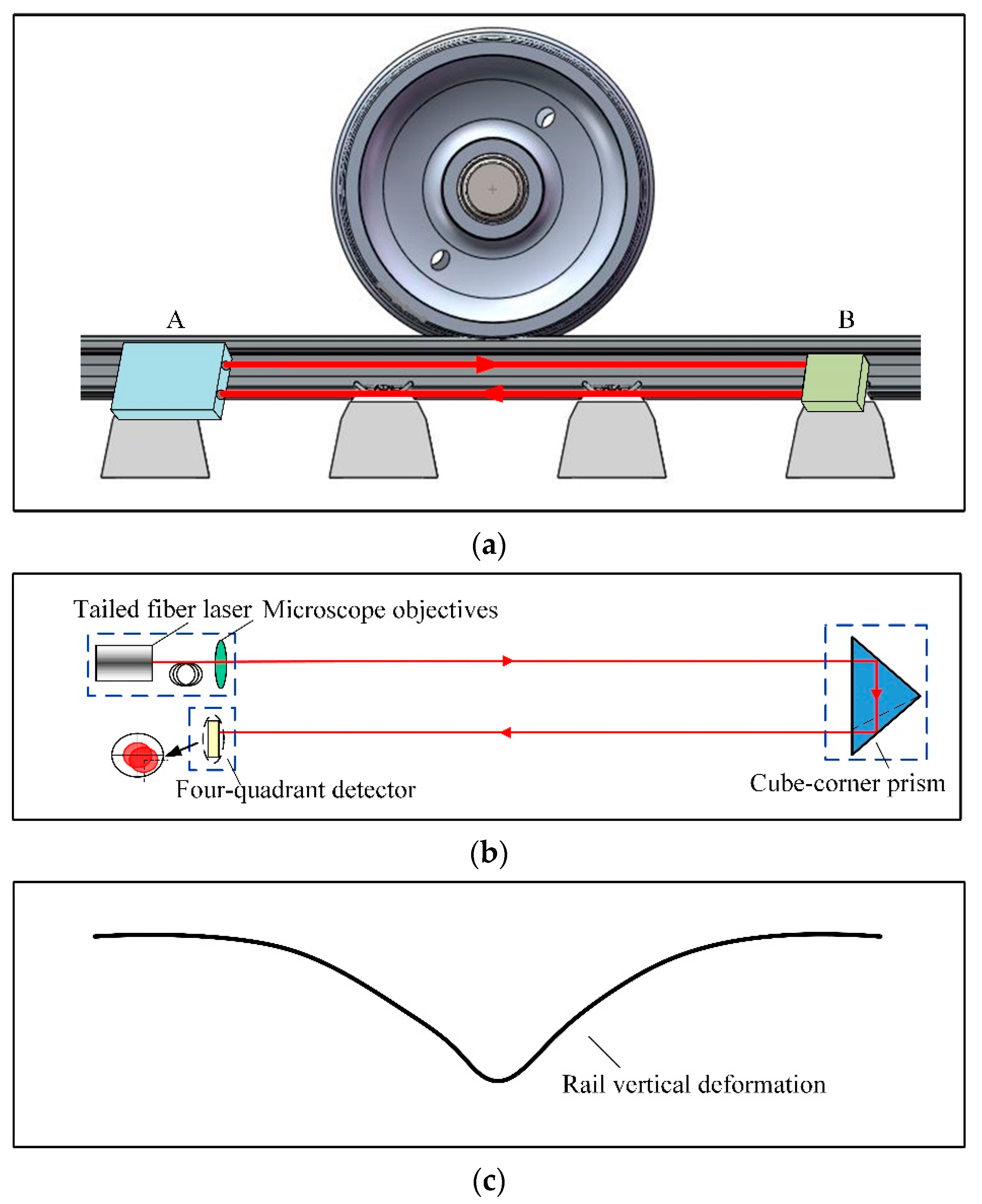
2. System Structure
2.1. Sensor Design
2.2. Measurement Principle
- (1)
- The vertical displacement of Part 1
- (2)
- Laser emission angle
- (3)
- The vertical displacement of Part 2
- (4)
- The angle of the cube-corner prism
- (5)
- Comprehensive analysis
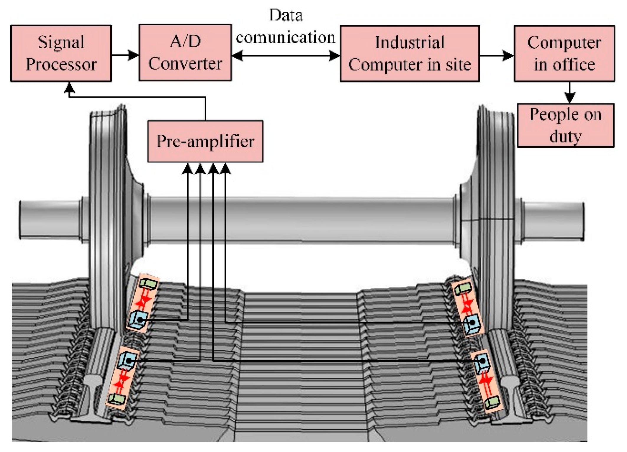
2.3. System Structure and Installation
3. Vehicle-Track Dynamics Simulation Model
3.1. The Vehicle Model
3.2. The Track Model
3.3. Mathematical Model of Wheel Flat
4. Dynamic Performance Analysis
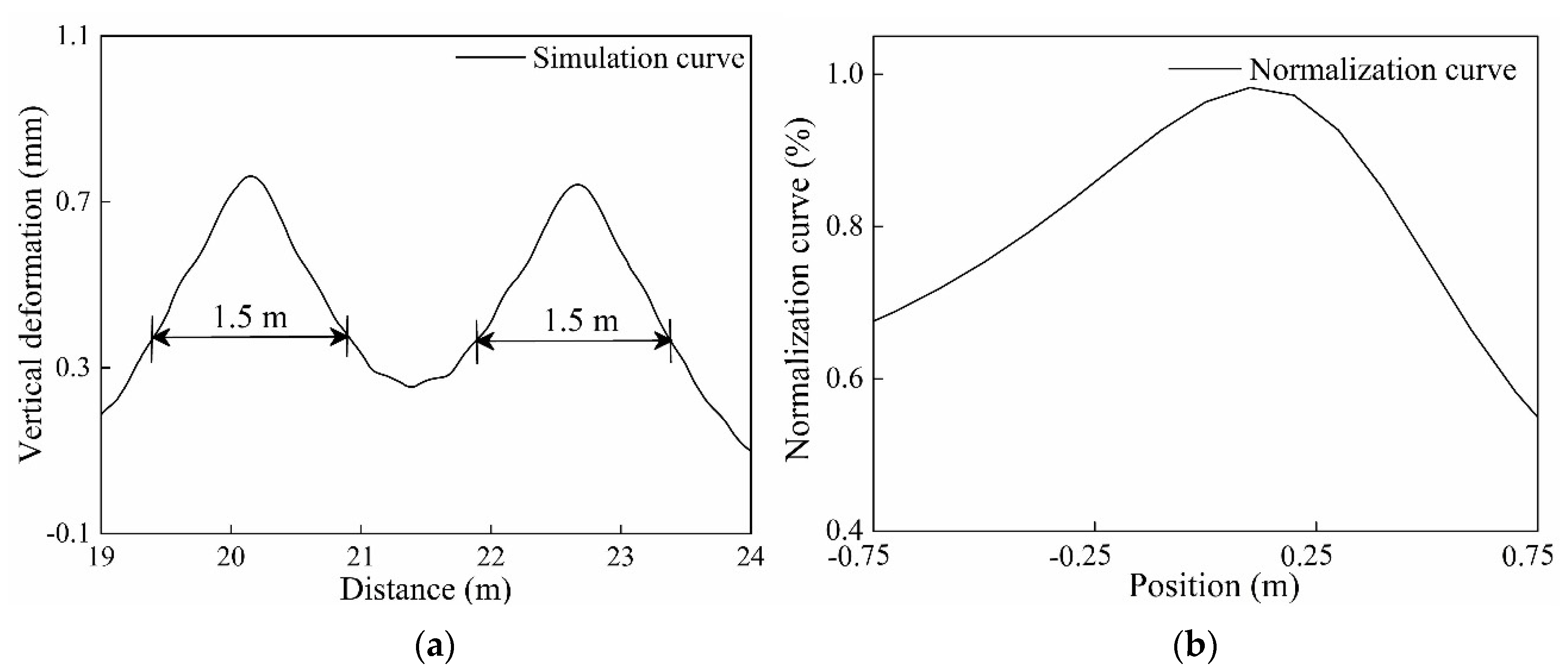
4.1. Rail Bending Deformation
4.2. Influence of Wheel Flat on Rail Deformation
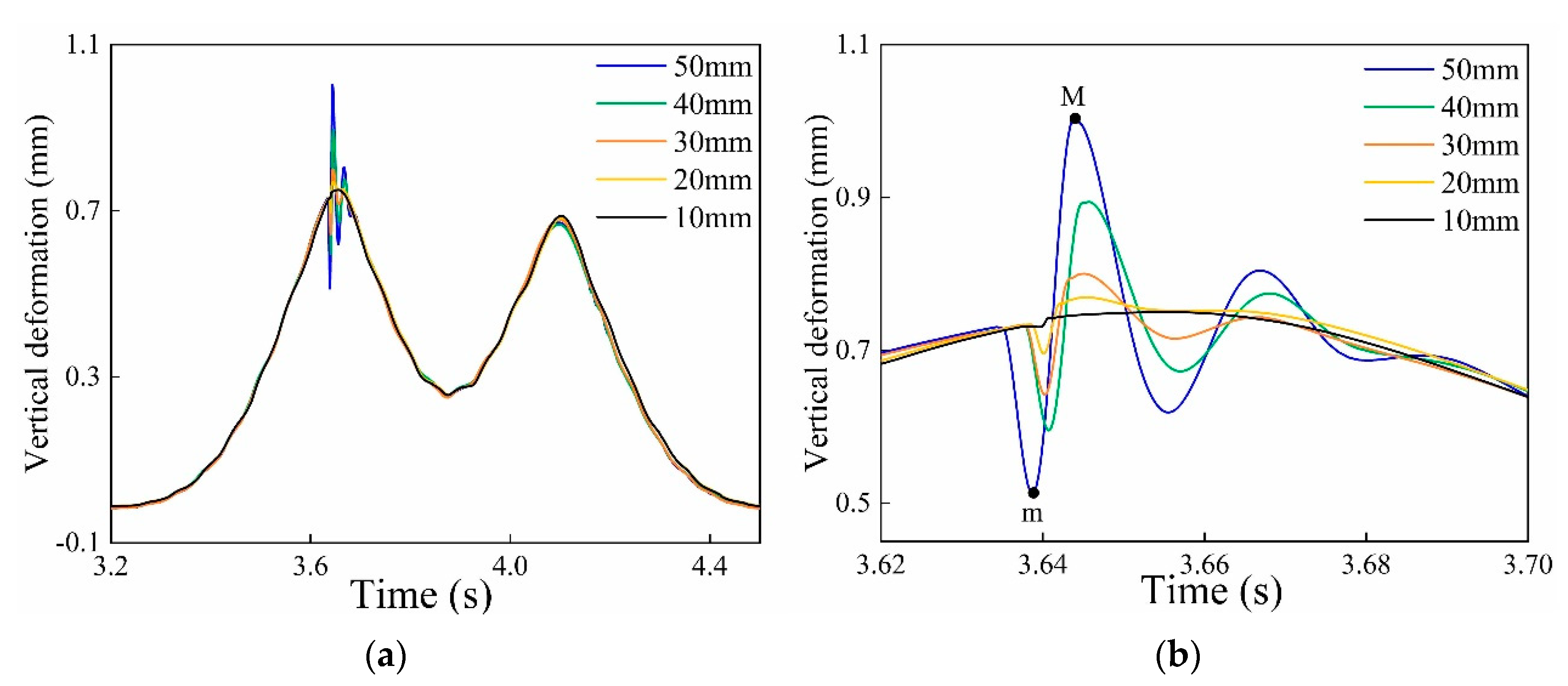
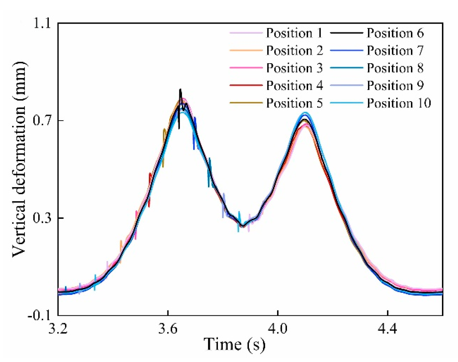
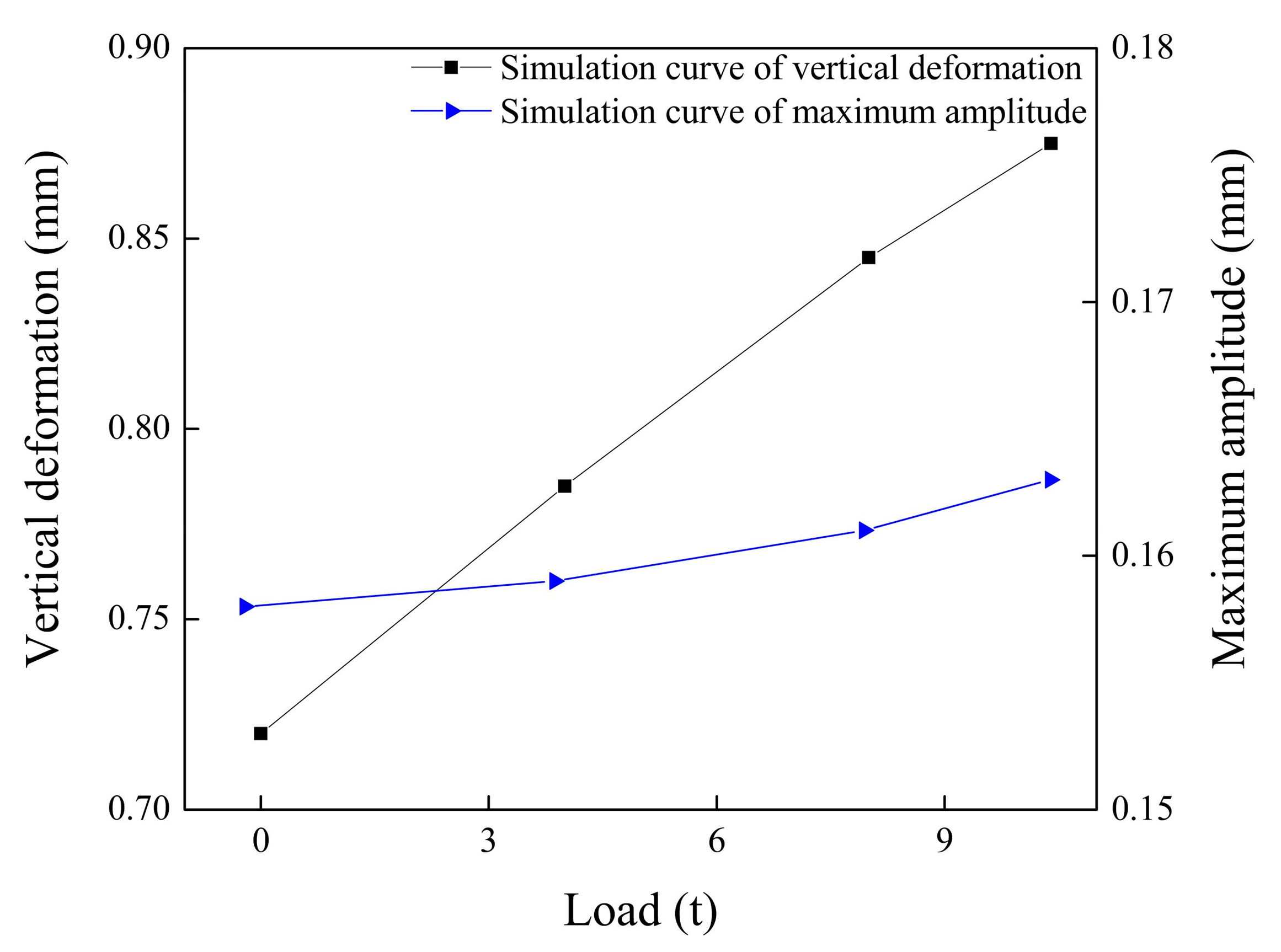
4.3. Analysis of Influencing Factors
4.4. The Quantification of Wheel Flat
5. Results and Discussion
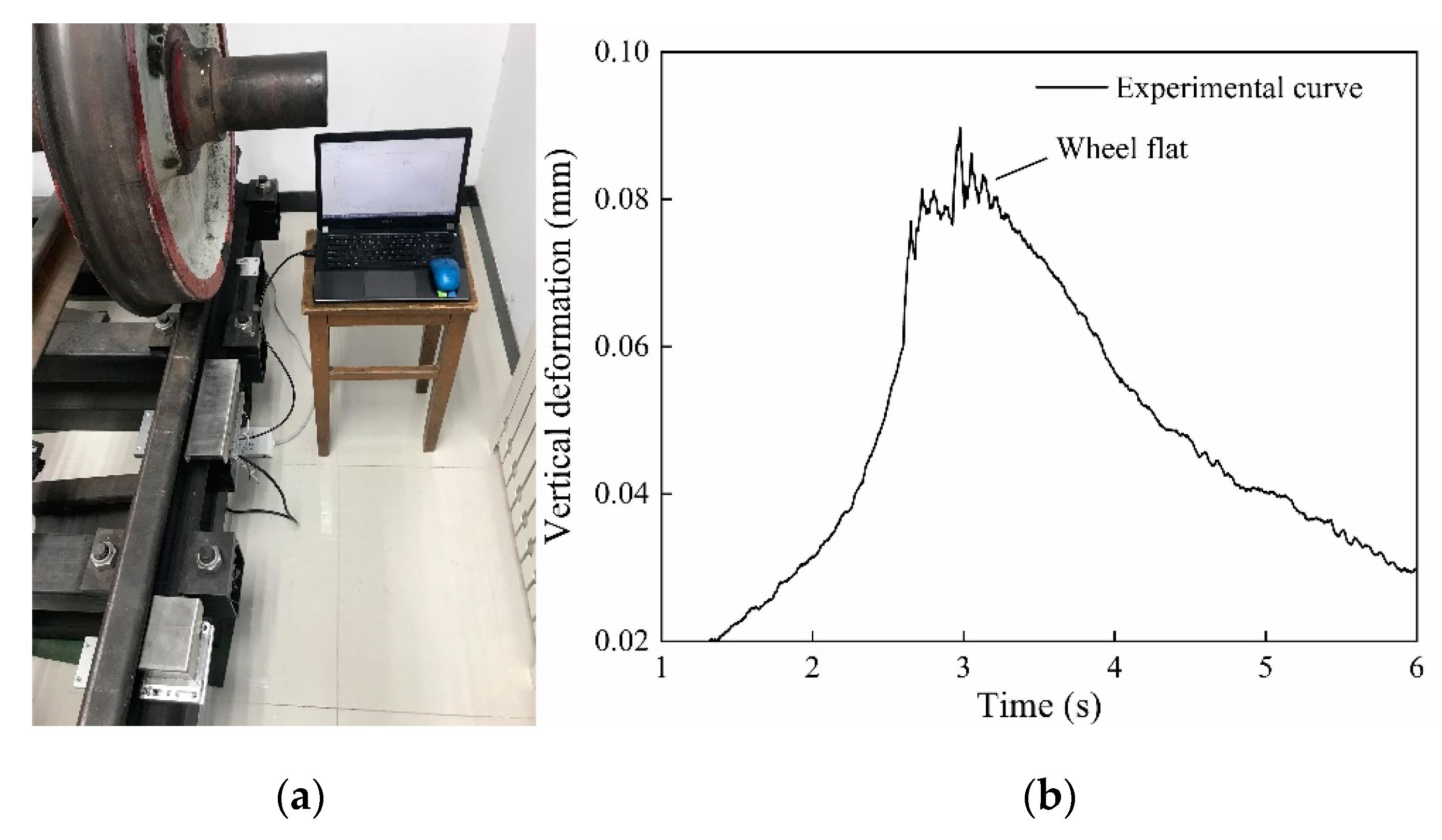
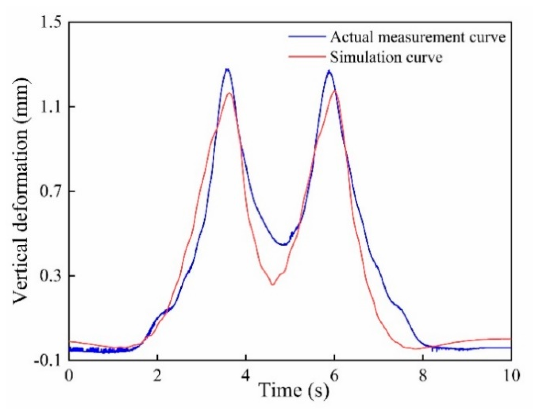
5.1. The Laboratory Experiment
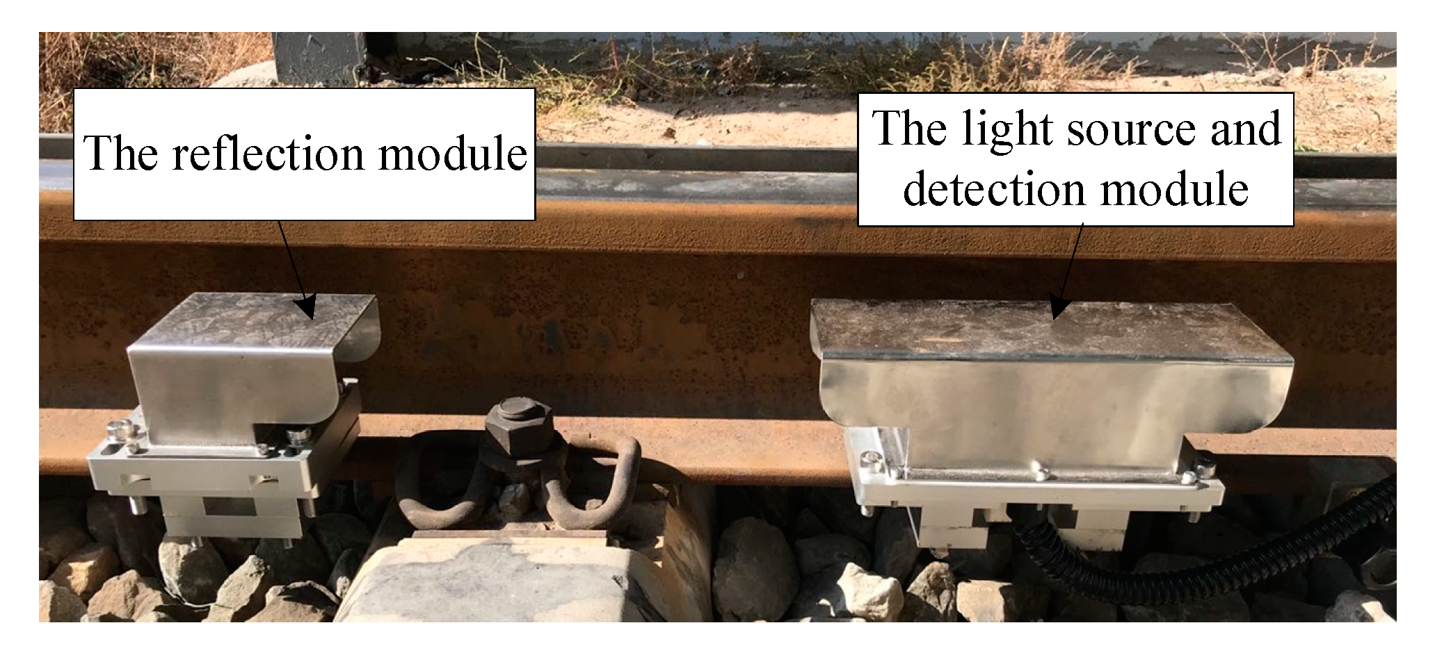
5.2. The Field Test
6. Conclusions
Author Contributions
Funding
Conflicts of Interest
References
- Ling, L.; Cao, Y.B.; Xiao, X.B.; Wen, Z.F.; Jin, X.S. Effect of Wheel Flats on the High-speed Wheel-Rail Contact Behavior. J. China Railw. Soc. 2015, 37, 32–39. [Google Scholar]
- Kumar, V.; Rastogi, V.; Pathak, P.M. Dynamic analysis of vehicle-track interaction due to wheel flat using bond graph. Proc. Inst. Mech. Eng. Part K J. Multi-Body Dyn. 2018, 232, 398–412. [Google Scholar] [CrossRef]
- Brizuela, J.; Fritsch, C.; Ibáñez, A. Railway wheel-flat detection and measurement by ultrasound. Transp. Res. Part C 2011, 19, 975–984. [Google Scholar] [CrossRef]
- Bogdevicius, M.; Zygiene, R.; Bureika, G.; Dailydka, S. An analytical mathematical method for calculation of the dynamic wheel–rail impact force caused by wheel flat. Veh. Syst. Dyn. 2016, 54, 689–705. [Google Scholar] [CrossRef]
- Bian, J.; Gu, Y.T.; Murray, M.H. A dynamic wheel–rail impact analysis of railway track under wheel flat by finite element analysis. Veh. Syst. Dyn. 2013, 51, 784–797. [Google Scholar] [CrossRef] [Green Version]
- Bogdevicius, M.; Zygiene, R.; Subacius, R. Employment of Two New Methods for the Research of Interaction of Wheel with a Flat and Rail. Solid State Phenom. 2017, 260, 289–294. [Google Scholar] [CrossRef]
- Keefe, R.; Ravitharan, S. Managing rail deterioration. In Proceedings of the International Conference Railway Engineering 2001, London, UK, 30 April–1 May 2001. [Google Scholar]
- Salzburger, H.J.; Schuppmann, M.; Wang, L.; Gao, X. In-Motion Ultrasonic Testing of the Tread of High-Speed Railway Wheels using the Inspection System AUROPA III. Insight-Non-Destr. Test. Cond. Monit. 2009, 51, 370–372. [Google Scholar] [CrossRef] [Green Version]
- Brizuela, J.; Ibáñez, A.; Nevado, P.; Fritsch, C. Railway wheels flat detector using Doppler effect. Phys. Procedia 2010, 3, 811–817. [Google Scholar] [CrossRef] [Green Version]
- Feng, Q.B.; Cui, J.Y.; Zhao, Y.; Pi, Y.; Teng, Y.P. A dynamic and quantitative method for measuring wheel flats and abrasion of trains. In Proceedings of the 5th WCDT World Conference on Non-Destructive Testing, Rome, Italy, 15–21 October 2000. [Google Scholar]
- Gao, R.; He, Q.X.; Feng, Q.B. Railway Wheel Flat Detection System Based on a Parallelogram Mechanism. Sensors 2019, 19, 3614. [Google Scholar] [CrossRef] [PubMed] [Green Version]
- Stratman, B.; Liu, Y.M.; Mahadevan, S. Structural Health Monitoring of Railroad Wheels Using Wheel Impact Load Detectors. J. Fail. Anal. Prev. 2007, 7, 218–225. [Google Scholar] [CrossRef]
- Zhang, Z.J.; Wei, S.H.; Andrawes, B.; Kuchma, D.A.; Edwards, J.R. Numerical and experimental study on dynamic behaviour of concrete sleeper track caused by wheel flat. Int. J. Rail Transp. 2016, 4, 1–19. [Google Scholar] [CrossRef]
- Li, Y.F.; Liu, J.X.; Wang, Y. Railway Wheel Flat Detection Based on Improved Empirical Mode Decomposition. Shock Vib. 2016, 2016, 1–14. [Google Scholar] [CrossRef]
- Li, Y.F.; Zuo, M.J.; Lin, J.H.; Liu, J.X. Fault detection method for railway wheel flat using an adaptive multiscale morphological filter. Mech. Syst. Signal Process. 2017, 84, 642–658. [Google Scholar] [CrossRef]
- Bosso, N.; Gugliotta, A.; Zampieri, N. Wheel Flat Detection Algorithm for Onboard Diagnostic. Measurement 2018, 123, 193–202. [Google Scholar] [CrossRef]
- Chudzikiewicz, A.; Bogacz, R.; Kostrzewski, M.; Konowrocki, R. Condition monitoring of railway track systems by using acceleration signals on wheelset axle-boxes. Transport 2018, 33, 555–566. [Google Scholar] [CrossRef] [Green Version]
- Belotti, V.; Crenna, F.; Michelini, R.C.; Rossi, G.B. Wheel-flat diagnostic tool via wavelet transform. Mech. Syst. Signal Process. 2006, 20, 1953–1966. [Google Scholar] [CrossRef]
- Lunys, O.; Dailydka, S.; Steišunas, S.; Bureika, G. Analysis of Freight Wagon Wheel Failure Detection in Lithuanian Railways. Procedia Eng. 2016, 134, 64–71. [Google Scholar] [CrossRef] [Green Version]
- Filograno, M.L.; Corredera, P.; Rodriguez-Plaza, M.; Andres-Alguacil, A.; Gonzalez-Herráez, M. Wheel Flat Detection in High-Speed Railway Systems Using Fiber Bragg Gratings. IEEE Sens. J. 2013, 13, 4808–4816. [Google Scholar] [CrossRef]
- Gao, X.; Guo, J. The detection of wheelflats based on fiber optic Bragg grating array. In Proceedings of the International Symposium on Precision Engineering Measurement & Instrumentation, Changsha, China, 6 March 2015. [Google Scholar]
- Iele, A.; Lopez, V.; Laudati, A.; Mazzino, N.; Cutolo, A. Fiber Optic Sensing System for Weighing In Motion (WIM) and Wheel Flat Detection (WFD) in railways assets: The TWBCS System. In Proceedings of the 8th European Workshop on Structural Health Monitoring (EWSHM 2016), Bilbao, Spain, 5–8 July 2016. [Google Scholar]
- Bracciali, A.; Lionetti, G.; Pieralli, M. Effective Wheel Flats Detection through a Simple Device. In Proceedings of the Techrail Workshop, Paris, France, 1 January 1997. [Google Scholar]
- Ren, Z.S.; Yang, G.; Wang, S.S.; Sun, S.G. Analysis of vibration and frequency transmission of high speed EMU with flexible model. Acta Mech. Sin. 2014, 30, 876–883. [Google Scholar] [CrossRef]


| Parameters | Values | Parameters | Values |
|---|---|---|---|
| Mass of car body (kg) | 4.72 104 | Pitch moment of inertia of bogie (kgm2) | 1205 |
| Mass of bogie (kg) | 3000 | Yaw moment of inertia of bogie (kgm2) | 2792 |
| Mass of wheel (kg) | 1900 | Vertical stiffness of primary suspension system [N/m] | 8.865 105 |
| Roll moment of inertia of car body (kgm2) | 9.25 104 | Vertical stiffness of secondary suspension system [N/m] | 2.03 105 |
| Pitch moment of inertia of car body (kgm2) | 1.756 105 | Vertical damping of primary suspension system[Ns/m] | 6 103 |
| Taw moment of inertia of car body (kgm2) | 1.728 105 | Vertical damping of secondary suspension system[Ns/m] | 8.4 104 |
| Roll moment of inertia of bogie (kgm2) | 1846 |
| Wheel Flat Length (mm) | |||||
|---|---|---|---|---|---|
| L = 18 | 0.0052 | 0.0051 | 0.0052 | 0.0054 | 0.0054 |
| L = 45 | 0.0157 | 0.0175 | 0.016 | 0.0168 | 0.0167 |
| L = 65 | 0.0184 | 0.0182 | 0.0189 | 0.0173 | 0.0182 |
© 2020 by the authors. Licensee MDPI, Basel, Switzerland. This article is an open access article distributed under the terms and conditions of the Creative Commons Attribution (CC BY) license (http://creativecommons.org/licenses/by/4.0/).
Share and Cite
Gao, R.; He, Q.; Feng, Q.; Cui, J. In-Service Detection and Quantification of Railway Wheel Flat by the Reflective Optical Position Sensor. Sensors 2020, 20, 4969. https://doi.org/10.3390/s20174969
Gao R, He Q, Feng Q, Cui J. In-Service Detection and Quantification of Railway Wheel Flat by the Reflective Optical Position Sensor. Sensors. 2020; 20(17):4969. https://doi.org/10.3390/s20174969
Chicago/Turabian StyleGao, Run, Qixin He, Qibo Feng, and Jianying Cui. 2020. "In-Service Detection and Quantification of Railway Wheel Flat by the Reflective Optical Position Sensor" Sensors 20, no. 17: 4969. https://doi.org/10.3390/s20174969
APA StyleGao, R., He, Q., Feng, Q., & Cui, J. (2020). In-Service Detection and Quantification of Railway Wheel Flat by the Reflective Optical Position Sensor. Sensors, 20(17), 4969. https://doi.org/10.3390/s20174969