3.1. Iterative K-Closest Point Algorithm for Pose Refinement
We present our algorithm for refining the rigid transformation from a source point cloud
to a reference point cloud
. The transformation is parameterized by a
rotation matrix
and a 3D translation vector
such that
for a corresponding pair
and
. We follow the general ICP framework, which alternates between correspondence-search and pose-estimation steps. One of the differences in our algorithm from the original ICP algorithm [
5] is that the correspondence is probabilistic. Unlike the fully probabilistic approaches [
11,
12], we assign matching probabilities only to the
K-closest points. Setting
K to a large number will increase the computational complexity while setting it to a small number will not produce a smoothed cost function that is easy to minimize [
11,
12]. In this paper, we set
K to 5 unless otherwise mentioned.
In the correspondence-search step, we perform a 6D search based on both 3D location and color [
8]. Each point
in
is transformed to
by using the current pose parameters
and
. Since we assume that the point clouds are obtained from RGB-D images, each point
is associated with its color vector
.
and
are joined together to produce a 6D vector
, where
is represented in the YIQ color space and then multiplied by a weight vector
for balancing between the two different quantities [
8]. The operation “∘” represents the Hadamard product. Such 6D vectors
are obtained from the reference points to build a
KD tree [
28] for accelerating the 6D search. The
K-nearest neighbors to
are then searched for, using the
KD tree.
Denoting the set of the
K-nearest neighbor indices as
, the
K-closest points are
for
. The residual vector
between
and
is defined as
Likewise, we define a 6D difference vector
as
We assume that has been sorted in ascending order of . The first element in , which is the nearest neighbor index, is denoted as for later use.
In the pose-estimation step, we find
and
that minimize the following cost:
where
is the matching probability between
and
such that either
or
for all
.
is a
matrix for defining the cost function as the sum of squared Mahalanobis distances in an arbitrary form. The factor
is for eliminating the factor 2 produced by differentiating the quadratic function.
Based on the assumption that the corresponding point is close to
in terms of both 3D location and color, we define
as
where
is the normalizing coefficient for ensuring the sum of
to be 1 unless all values of
are 0.
is the distance threshold typically employed in most ICP algorithms. In this paper, we use a user-defined value, which will be specified later in this section. If the median of
is greater than
for the initial pose parameters
and
then
is replaced with the median. This is intended to provide a sufficient number of correspondences if the initial registration error is large.
is set to
.
Throughout this paper, we assume that the initial pose parameters
and
are given. In practice, we can employ global registration algorithms [
18,
19,
20,
21] to estimate them. For a multi-view system, they can be estimated by calibrating the camera network [
34].
The state-of-the-art cost functions are defined as the sum of squared point-to-plane [
6,
24] or plane-to-plane distances [
10,
13]. For the plane-to-plane distances,
depends on both source and reference points and needs to be recomputed after every correspondence-search step. In contrast, for the point-to-plane distances,
depends only on reference points and needs to be computed only once. In this case,
is defined as
where
is the surface normal vector of
.
The rank of
is 1 and thus
is noninvertible. To increase the numerical stability of our optimization algorithm, we add
to
, where
is a small positive number (0.001 in this paper). Our
is defined as
Defining in this form is also equivalent to defining the cost function as the weighted sum of squared point-to-point and point-to-plane distances.
To minimize
E in Equation (
4), we apply the Gauss–Newton algorithm, which is widely employed in ICP variants [
24,
25,
35]. During the minimization,
is regarded as a fixed variable although it depends on the pose parameters. We use the approximation form for an incremental rotation [
35] as defined by
where
,
, and
are the rotation angles about
X,
Y, and
Z axes, respectively. Denoting an incremental translation by
, the incremental transformation parameters can be represented by a vector
.
Let us define
as
computed with the current rotation and translation parameters.
is then approximated by
where
is the
Jacobian matrix with the partial derivatives of
with respect to the components of
:
The gradient of
E is then computed as
Solving for
satisfying
gives
The new rotation matrix and translation vector is computed as
is updated using the new pose parameters and the Gauss–Newton step is iteratively applied until convergence. The algorithm is configured to terminate when the magnitudes of the incremental rotation and translation are below threshold levels or when a maximum iteration count is reached. The thresholds are set to rotation and 0.001 mm translation with a maximum iteration count of 80.
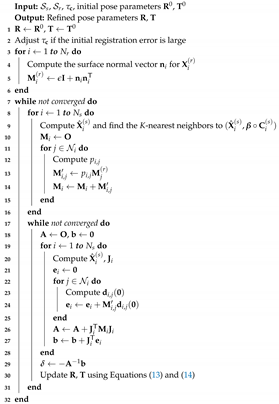
Algorithm 1 summarizes the presented algorithm for pose refinement.
| Algorithm 1: Iterative K-closest point algorithm for pose refinement. |
![Sensors 20 05331 i001]() |
Since our pose refinement algorithm is a local registration algorithm, a good initial pose is necessary to converge to an accurate pose. To alleviate getting trapped in local minima, probabilistic approaches rely on annealing schemes [
6,
12]. In this paper, we rely on a coarse-to-fine scheme [
24]. Three pairs of point clouds of different resolutions are built by downsampling input source and reference point clouds using voxel grids with voxel sizes of 4, 2, and 1 cm. The output from a coarse level is used as the input initial pose parameters to the adjacent finer level. Our assumption of small
and
may not hold in coarse levels because we cannot guarantee the quality of the initial alignment. Thus, we set
to
in the two coarse levels. The resulting cost function can be minimized by finding the direct solution to a weighted least squares problem [
36]. For each level,
is set to
times the voxel size.
The downsampling in the coarse-to-fine scheme is similar to the decimation in the annealing scheme of the multiscale EM-ICP algorithm [
12]. The scale parameter in [
12] has a similar meaning to the voxel size. With a small number of data points at a coarse level, the shape of the cost function becomes simple and easy to minimize. Although the optimal solution of a coarse level tends to be shifted from the optimal solution to the original cost function [
12], it can be a good initial solution for the next level. This coarse-to-fine scheme cannot deal with an arbitrary initial pose, but it was shown to be efficient and effective in practice [
24].
3.2. Iterative K-Closest Point Algorithm for Depth Refinement
An interesting discovery of this paper is that the alignment between two point clouds can also be achieved by refining the measured depth values. Regarding the measured depth value
of a point
as a variable, we can solve for
minimizing Equation (
4). Regarding
and
as constants,
E can be considered as the sum of independent cost functions
:
where
Denoting the normalized image coordinate vector [
22] corresponding to
as
,
equals
. The gradient of
with respect to
is computed as
By applying the chain rule, the derivative of
with respect to
is computed as
Solving for
satisfying
yields to
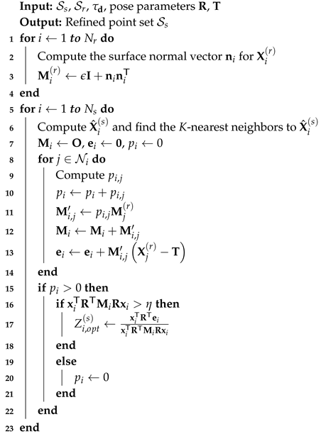
Algorithm 2 summarizes the presented algorithm for depth refinement. In the depth refinement step, we assume that the pose refinement algorithm has aligned the point clouds, so we perform the conventional 3D search in Algorithm 2. We use a spatial distance threshold
cm to prevent a spatially distant point from becoming a neighbor to
. However, we use the same weighting function in Equation (
5) to allow similarly colored point pairs to have high
. In Equation (
5), the condition
is replaced with
based on the 3D search.
| Algorithm 2: Iterative K-closest point algorithm for depth refinement. |
![Sensors 20 05331 i002]() |
In Algorithm 2, is a positive constant for ensuring the numerical stability of the division. For some points, can be greater than . In this case, is set to either or to restrict the change to be local.
Not all source points may find their closest points within the threshold level. In this case, source points without valid closest points can not be changed by Algorithm 2. To attract the unchanged points to the refined points, we minimize the following cost
F instead of directly replacing
with
.
where
, which is either 1 or 0, is an indicator of valid
for
.
is the initial difference
before minimizing
F.
is the eight neighbors’ indices around the pixel location of
in the image.
Applying the Jacobi method to minimization of
F yields to the following update equation:
where
is a weight for balancing between the two different terms, which is set to 0.2 throughout this paper.
is the number of elements in
. For
with
, a neighboring updated
pulls
toward
by an amount of
preserving the initial relative difference. The update equation is applied to all source points six times. This small maximum iteration count is appropriate if the source fragment is a proper subset of the reference fragment. For this reason, we apply the presented algorithm only to the merged point cloud described in the next section.


