A Patient-Specific 3D+t Coronary Artery Motion Modeling Method Using Hierarchical Deformation with Electrocardiogram


Abstract
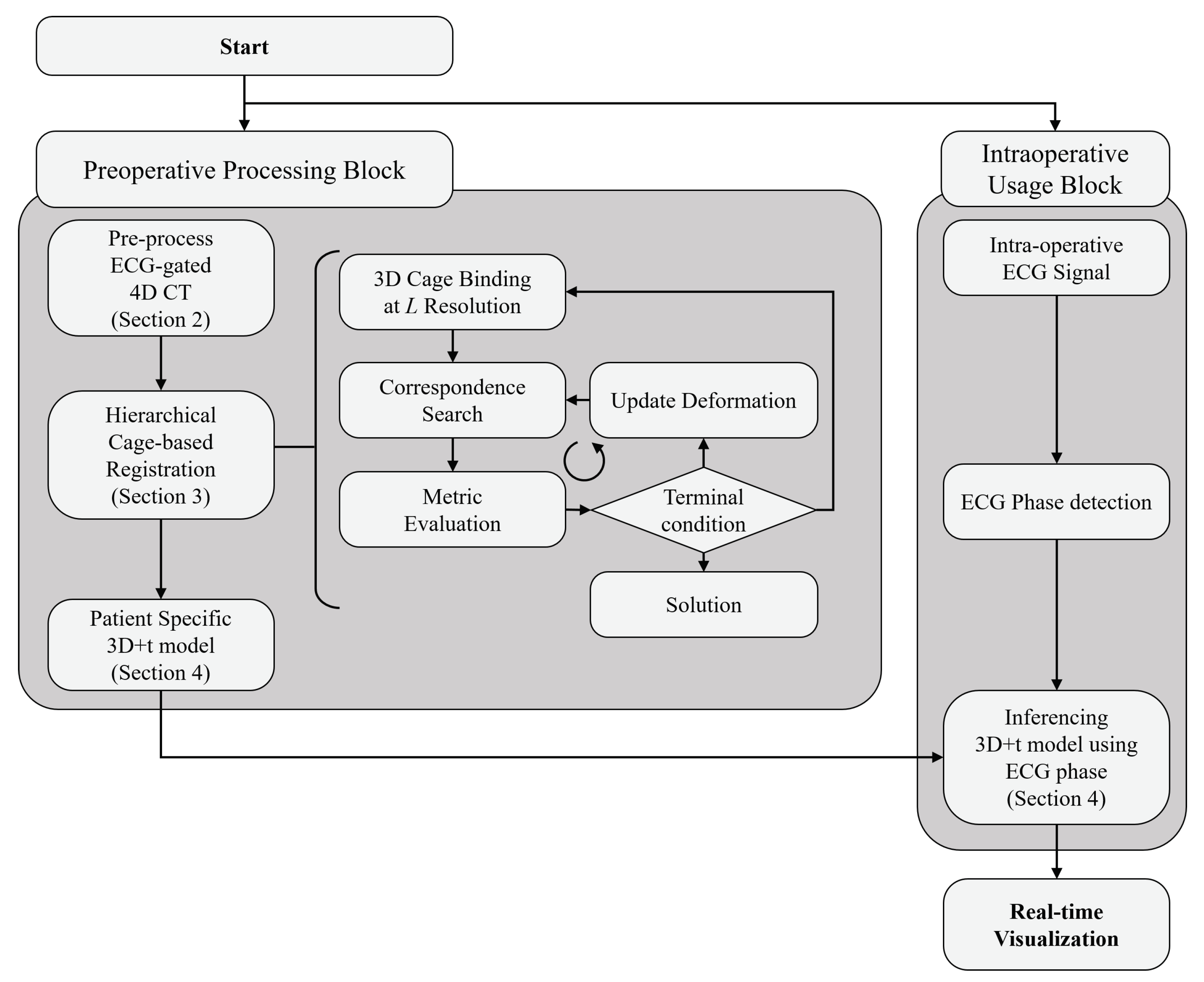
:1. Introduction
- A hierarchical deformation method to perform robust shape registration, even with incomplete coronary artery models;
- Rapid shape interpolation that enables restoring small and complex geometry in a time-varying coronary artery model;
- The modified hyper-elastic regularization prevents mesh degeneration during shape registration; and
- Evaluation of the proposed method using retrospective data for eight patients, both qualitatively and quantitatively.
2. Pre-Processing ECG-Gated 4D CT Images
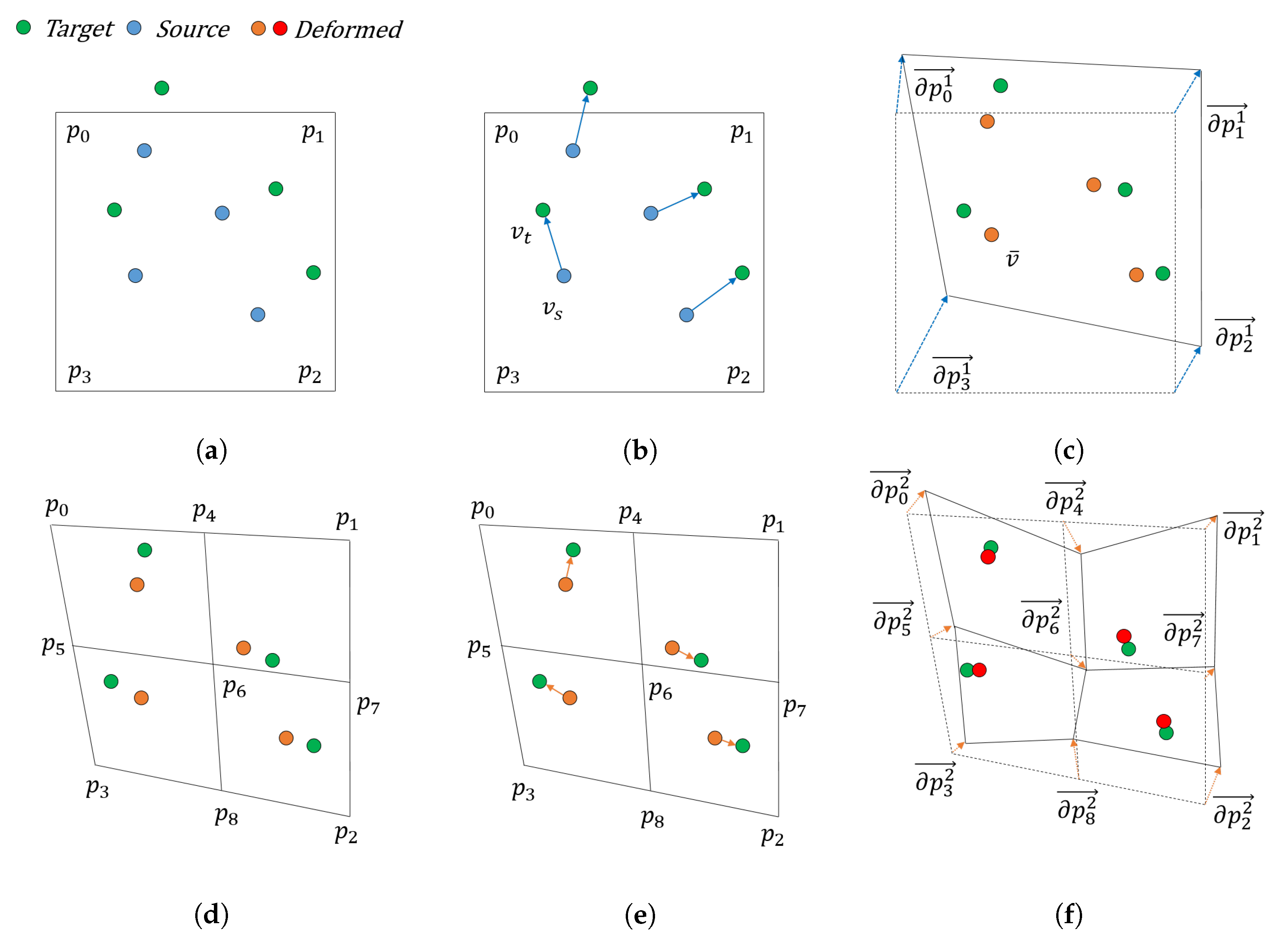
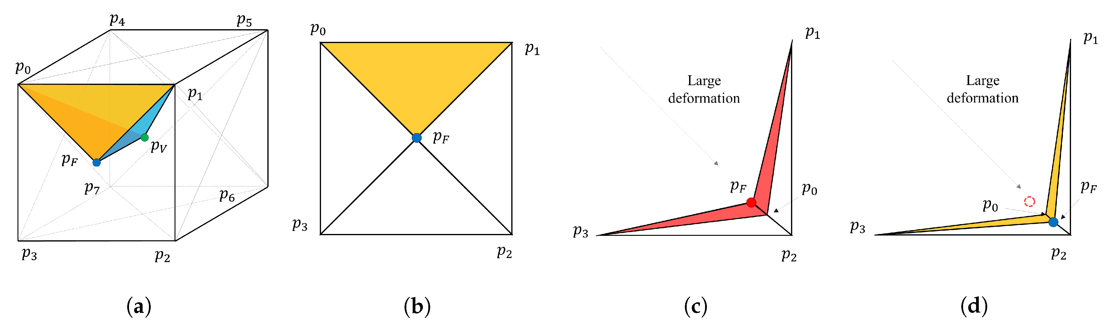
3. Hierarchical Cage-Based Shape Registration Method
3.1. Shape Representation and Registration Problems
3.2. Gradient Descent for Shape Control Point Optimization
3.3. Multi-Resolution Cage Deformation Representation
3.4. Diffeomorphism Supported by Hyper-Elasticity Regularization
4. Interpolation of Shape Control Points
5. Evaluations and Results
5.1. Quantitative Evaluations
5.1.1. Trade-off between Deformation Depth and Computation Time
5.1.2. Comparison with Other Methods
5.1.3. Interpolation Accuracy
5.2. Qualitative Evaluations
5.2.1. The Effect of Hyper-Elastic Regularization and Hierarchical Deformation
5.2.2. The Representation Power of Interpolated Model
6. Discussion and Conclusions
- The trade-off between the shape matching accuracy and calculation time according to the hierarchical deformation;
- The comparative evaluation with other methods;
- The accuracy of the shape interpolation model, according to the time sampling interval.
Author Contributions
Funding
Conflicts of Interest
Appendix A. Patient-Wise Evaluations
Appendix A.1. Dice Coefficients at Different Levels of Deformation

Appendix A.2. Average Distances at Different Levels of Deformation

Appendix A.3. Dice Coefficients for Different Methods

Appendix A.4. Average Distances for Different Methods

Appendix A.5. Dice Coefficients for Different Phase Sampling Methods

Appendix A.6. Average Distances for Different Phase Sampling Methods

References
- Virani, S.S.; Alonso, A.; Benjamin, E.J.; Bittencourt, M.S.; Callaway, C.W.; Carson, A.P.; Chamberlain, A.M.; Chang, A.R.; Cheng, S.; Delling, F.N.; et al. Heart disease and stroke statistics—2020 update a report from the American Heart Association. Circulation 2020, E139–E596. [Google Scholar] [CrossRef] [PubMed]
- Hadjiiski, L.; Zhou, C.; Chan, H.P.; Chughtai, A.; Agarwal, P.; Kuriakose, J.; Kazerooni, E.; Wei, J.; Patel, S. Coronary CT angiography (cCTA): Automated registration of coronary arterial trees from multiple phases. Phys. Med. Biol. 2014, 59, 4661. [Google Scholar] [CrossRef] [PubMed] [Green Version]
- Zeng, S.; Feng, J.; An, Y.; Lu, B.; Lu, J.; Zhou, J. Towards Accurate and Complete Registration of Coronary Arteries in CTA Images. In Proceedings of the International Conference on Medical Image Computing and Computer-Assisted Intervention, Granada, Spain, 16–20 September 2018; pp. 419–427. [Google Scholar]
- Biglarian, M.; Larimi, M.M.; Afrouzi, H.H.; Moshfegh, A.; Toghraie, D.; Javadzadegan, A.; Rostami, S. Computational investigation of stenosis in curvature of coronary artery within both dynamic and static models. Comput. Meth. Programs Biomed. 2020, 185, 105170. [Google Scholar] [CrossRef] [PubMed]
- Wu, X.; von Birgelen, C.; Muramatsu, T.; Li, Y.; Holm, N.R.; Reiber, J.H.; Tu, S. A novel four-dimensional angiographic approach to assess dynamic superficial wall stress of coronary arteries in vivo: Initial experience in evaluating vessel sites with subsequent plaque rupture. EuroIntervention 2017, 13, e1099–e1103. [Google Scholar] [CrossRef] [Green Version]
- Elattar, M.A.; Vink, L.W.; van Mourik, M.S.; Baan Jr, J.; vanBavel, E.T.; Planken, R.N.; Marquering, H.A. Dynamics of the aortic annulus in 4D CT angiography for transcatheter aortic valve implantation patients. PLoS ONE 2017, 12, e0184133. [Google Scholar] [CrossRef] [Green Version]
- Shi, B.; Katsevich, G.; Chiang, B.S.; Katsevich, A.; Zamyatin, A. Image registration for motion estimation in cardiac CT. In Proceedings of the 2014 SPIE Medical Imaging, San Diego, CA, USA, 15–20 February 2014; Volume 9033, p. 90332E. [Google Scholar]
- Forte, M.N.V.; Valverde, I.; Prabhu, N.; Correia, T.; Narayan, S.A.; Bell, A.; Mathur, S.; Razavi, R.; Hussain, T.; Pushparajah, K.; et al. Visualization of coronary arteries in paediatric patients using whole-heart coronary magnetic resonance angiography: Comparison of image-navigation and the standard approach for respiratory motion compensation. J. Cardiovasc. Magn. Reson. 2019, 21, 1–9. [Google Scholar]
- Coppo, S.; Piccini, D.; Bonanno, G.; Chaptinel, J.; Vincenti, G.; Feliciano, H.; Van Heeswijk, R.B.; Schwitter, J.; Stuber, M. Free-running 4D whole-heart self-navigated golden angle MRI: Initial results. Magn. Reson. Med. 2015, 74, 1306–1316. [Google Scholar] [CrossRef]
- Li, S.; Xie, Z.; Xia, Q.; Hao, A.; Qin, H. Hybrid 4D cardiovascular modeling based on patient-specific clinical images for real-time PCI surgery simulation. Graph. Model. 2019, 101, 1–7. [Google Scholar] [CrossRef]
- Lamash, Y.; Fischer, A.; Carasso, S.; Lessick, J. Strain analysis from 4-D cardiac CT image data. IEEE Trans. Biomed. Eng. 2014, 62, 511–521. [Google Scholar] [CrossRef]
- Gupta, V.; Lantz, J.; Henriksson, L.; Engvall, J.; Karlsson, M.; Persson, A.; Ebbers, T. Automated three-dimensional tracking of the left ventricular myocardium in time-resolved and dose-modulated cardiac CT images using deformable image registration. J. Cardiovasc. Comput. Tomogr. 2018, 12, 139–148. [Google Scholar]
- Li, Q.; Tong, Y.; Yin, Y.; Cheng, P.; Gong, G. Definition of the margin of major coronary artery bifurcations during radiotherapy with electrocardiograph-gated 4D-CT. Phys. Med. 2018, 49, 90–94. [Google Scholar] [CrossRef] [PubMed] [Green Version]
- Liu, B.; Bai, X.; Zhou, F. Local motion-compensated method for high-quality 3D coronary artery reconstruction. Biomed. Opt. Express 2016, 7, 5268–5283. [Google Scholar] [CrossRef] [PubMed] [Green Version]
- Chen, M.Y.; Shanbhag, S.M.; Arai, A.E. Submillisievert median radiation dose for coronary angiography with a second-generation 320–detector row CT scanner in 107 consecutive patients. Radiology 2013, 267, 76–85. [Google Scholar] [CrossRef] [PubMed] [Green Version]
- Besl, P.J.; McKay, N.D. Method for registration of 3-D shapes. In Proceedings of the Robotics ’91, Boston, MA, USA, 14–15 November 1991. [Google Scholar]
- Sorkine, O.; Alexa, M. As-rigid-as-possible surface modeling. In Proceedings of the Symposium on Geometry Processing, Barcelona, Spain, 4–6 July 2007; Volume 4, pp. 109–116. [Google Scholar]
- Davatzikos, C. Spatial transformation and registration of brain images using elastically deformable models. Comput. Vis. Image Underst. 1997, 66, 207–222. [Google Scholar] [CrossRef] [Green Version]
- Pennec, X.; Stefanescu, R.; Arsigny, V.; Fillard, P.; Ayache, N. Riemannian elasticity: A statistical regularization framework for non-linear registration. In Proceedings of the International Conference on Medical Image Computing and Computer-Assisted Intervention, Palm Springs, CA, USA, 26–29 October 2005; pp. 943–950. [Google Scholar]
- Burger, M.; Modersitzki, J.; Ruthotto, L. A hyperelastic regularization energy for image registration. SIAM J. Sci. Comput. 2013, 35, B132–B148. [Google Scholar] [CrossRef]
- Chiang, M.C.; Leow, A.D.; Klunder, A.D.; Dutton, R.A.; Barysheva, M.; Rose, S.E.; McMahon, K.L.; De Zubicaray, G.I.; Toga, A.W.; Thompson, P.M. Fluid registration of diffusion tensor images using information theory. IEEE Trans. Med. Imaging 2008, 27, 442–456. [Google Scholar] [CrossRef] [Green Version]
- Vercauteren, T.; Pennec, X.; Perchant, A.; Ayache, N. Symmetric log-domain diffeomorphic registration: A demons-based approach. In Proceedings of the International Conference on Medical Image Computing and Computer-Assisted Intervention, New York, NY, USA, 6–10 September 2008; pp. 754–761. [Google Scholar]
- Yeo, B.T.; Vercauteren, T.; Fillard, P.; Peyrat, J.M.; Pennec, X.; Golland, P.; Ayache, N.; Clatz, O. DT-REFinD: Diffusion tensor registration with exact finite-strain differential. IEEE Trans. Med. Imaging 2009, 28, 1914–1928. [Google Scholar] [CrossRef] [Green Version]
- Younes, L.; Qiu, A.; Winslow, R.L.; Miller, M.I. Transport of relational structures in groups of diffeomorphisms. J. Math. Imaging Vis. 2008, 32, 41–56. [Google Scholar] [CrossRef] [Green Version]
- Cootes, T.F.; Taylor, C.J.; Cooper, D.H.; Graham, J. Active shape models-their training and application. Comput. Vis. Image Underst. 1995, 61, 38–59. [Google Scholar] [CrossRef] [Green Version]
- Glocker, B.; Komodakis, N.; Navab, N.; Tziritas, G.; Paragios, N. Dense registration with deformation priors. In Proceedings of the International Conference on Information Processing in Medical Imaging, Williamsburg, VA, USA, 5–10 July 2009; pp. 540–551. [Google Scholar]
- Baka, N.; Metz, C.; Schultz, C.; Neefjes, L.; van Geuns, R.J.; Lelieveldt, B.P.; Niessen, W.J.; van Walsum, T.; de Bruijne, M. Statistical coronary motion models for 2D+ t/3D registration of X-ray coronary angiography and CTA. Med. Image Anal. 2013, 17, 698–709. [Google Scholar] [CrossRef]
- Yang, X.; Xue, Z.; Liu, X.; Xiong, D. Topology preservation evaluation of compact-support radial basis functions for image registration. Pattern Recognit. Lett. 2011, 32, 1162–1177. [Google Scholar] [CrossRef]
- Donato, G.; Belongie, S. Approximate thin plate spline mappings. In Proceedings of the European Conference on Computer Vision, Copenhagen, Denmark, 28–31 May 2002; pp. 21–31. [Google Scholar]
- Sederberg, T.W.; Parry, S.R. Free-form deformation of solid geometric models. In Proceedings of the 13th Annual Conference on Computer Graphics and Interactive Techniques, Dallas, TX, USA, 18–22 August 1986; pp. 151–160. [Google Scholar]
- Sdika, M. A fast nonrigid image registration with constraints on the Jacobian using large scale constrained optimization. IEEE Trans. Med. Imaging 2008, 27, 271–281. [Google Scholar] [CrossRef] [PubMed]
- Rueckert, D.; Aljabar, P.; Heckemann, R.A.; Hajnal, J.V.; Hammers, A. Diffeomorphic registration using B-splines. In Proceedings of the International Conference on Medical Image Computing and Computer-Assisted Intervention, Copenhagen, Denmark, 1–6 October 2006; pp. 702–709. [Google Scholar]
- Chui, H.; Rangarajan, A. A new point matching algorithm for non-rigid registration. Comput. Vis. Image Underst. 2003, 89, 114–141. [Google Scholar] [CrossRef]
- Chui, H.; Rangarajan, A. A feature registration framework using mixture models. In Proceedings of the IEEE Workshop on Mathematical Methods in Biomedical Image Analysis (MMBIA-2000), Hilton Head Island, SC, USA, 11–12 June 2000; pp. 190–197. [Google Scholar]
- Jian, B.; Vemuri, B.C. A robust algorithm for point set registration using mixture of Gaussians. In Proceedings of the 10th IEEE International Conference on Computer Vision (ICCV’05), Las Vegas, NV, USA, 17–21 October 2005; pp. 1246–1251. [Google Scholar]
- Myronenko, A.; Song, X.; Carreira-Perpinán, M.A. Non-rigid point set registration: Coherent point drift (CPD). Adv. Neural Inf. Process. Syst. 2007, 1, 1009–1016. [Google Scholar]
- Myronenko, A.; Song, X. Point set registration: Coherent point drift. IEEE Trans. Pattern Anal. Mach. Intell. 2010, 32, 2262–2275. [Google Scholar] [CrossRef] [PubMed] [Green Version]
- Jian, B.; Vemuri, B.C. Robust point set registration using gaussian mixture models. IEEE Trans. Pattern Anal. Mach. Intell. 2010, 33, 1633–1645. [Google Scholar] [CrossRef]
- Ma, J.; Qiu, W.; Zhao, J.; Ma, Y.; Yuille, A.L.; Tu, Z. Robust L2E estimation of transformation for non-rigid registration. IEEE Trans. Signal Process. 2015, 63, 1115–1129. [Google Scholar] [CrossRef]
- Ma, J.; Zhao, J.; Yuille, A.L. Non-rigid point set registration by preserving global and local structures. IEEE Trans. Image Process. 2015, 25, 53–64. [Google Scholar]
- Yushkevich, P.A.; Piven, J.; Cody Hazlett, H.; Gimpel Smith, R.; Ho, S.; Gee, J.C.; Gerig, G. User-Guided 3D Active Contour Segmentation of Anatomical Structures: Significantly Improved Efficiency and Reliability. Neuroimage 2006, 31, 1116–1128. [Google Scholar] [CrossRef] [Green Version]
- Seifarth, H.; Wienbeck, S.; Pusken, M.; Juergens, K.U.; Maintz, D.; Vahlhaus, C.; Heindel, W.; Fischbach, R. Optimal systolic and diastolic reconstruction windows for coronary CT angiography using dual-source CT. Am. J. Roentgenol. 2007, 189, 1317–1323. [Google Scholar] [CrossRef]
- Press, W.H.; Teukolsky, S.A.; Vetterling, W.T.; Flannery, B.P. Numerical Recipes 3rd Edition: The Art of Scientific Computing; Cambridge University Press: New York, NY, USA, 2007. [Google Scholar]
- Dagum, L.; Ramesh, M. OpenMP: An industry standard API for shared-memory programming. IEEE Comput. Sci. Eng. 1998, 5, 46–55. [Google Scholar] [CrossRef] [Green Version]
- Pheatt, C. Intel® threading building blocks. J. Comput. Sci. Coll. 2008, 23, 298. [Google Scholar]


| Method | Cage Resolution | Computation Time (s) | Average Distance (mm) | Dice Coefficient |
|---|---|---|---|---|
| HierCage | [1, 1, 1] | 21.73 | 0.668 ± 0.255 | 0.655 ± 0.096 |
| HierCage | [2, 2, 2] | 23.05 | 0.597 ± 0.234 | 0.696 ± 0.077 |
| HierCage | [3, 3, 3] | 22.91 | 0.566 ± 0.227 | 0.721 ± 0.068 |
| HierCage | [4, 4, 4] | 23.52 | 0.543 ± 0.222 | 0.735 ± 0.064 |
| HierCage | [5, 5, 5] | 33.00 | 0.534 ± 0.221 | 0.741 ± 0.064 |
| GRBF_KC | [4, 4, 4] | 40.99 | 0.615 ± 0.218 | 0.666 ± 0.088 |
| GRBF_L2 | [4, 4, 4] | 40.92 | 0.600 ± 0.207 | 0.671 ± 0.084 |
| TPS_KC | [4, 4, 4] | 33.00 | 0.553 ± 0.191 | 0.681 ± 0.080 |
| TPS_L2 | [4, 4, 4] | 32.21 | 0.530 ± 0.17 | 0.690 ± 0.075 |
© 2020 by the authors. Licensee MDPI, Basel, Switzerland. This article is an open access article distributed under the terms and conditions of the Creative Commons Attribution (CC BY) license (http://creativecommons.org/licenses/by/4.0/).
Share and Cite
Yoon, S.; Yoon, C.; Chun, E.J.; Lee, D. A Patient-Specific 3D+t Coronary Artery Motion Modeling Method Using Hierarchical Deformation with Electrocardiogram. Sensors 2020, 20, 5680. https://doi.org/10.3390/s20195680
Yoon S, Yoon C, Chun EJ, Lee D. A Patient-Specific 3D+t Coronary Artery Motion Modeling Method Using Hierarchical Deformation with Electrocardiogram. Sensors. 2020; 20(19):5680. https://doi.org/10.3390/s20195680
Chicago/Turabian StyleYoon, Siyeop, Changhwan Yoon, Eun Ju Chun, and Deukhee Lee. 2020. "A Patient-Specific 3D+t Coronary Artery Motion Modeling Method Using Hierarchical Deformation with Electrocardiogram" Sensors 20, no. 19: 5680. https://doi.org/10.3390/s20195680