The detected objects in solid–liquid two-phase flow can be categorized into distinguishable and undistinguishable types by ERT, and accordingly, our proposed method is illustrated by two cases.
3.1. Computation on Distinguishable Objects by the Fast Fuzzy Cluster Algorithm (f-FCM) Algorithm
If all detected objects in a field have a large enough size, these objects can be distinguished in an ERT image.
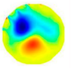
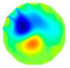
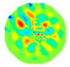
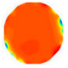
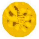
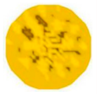
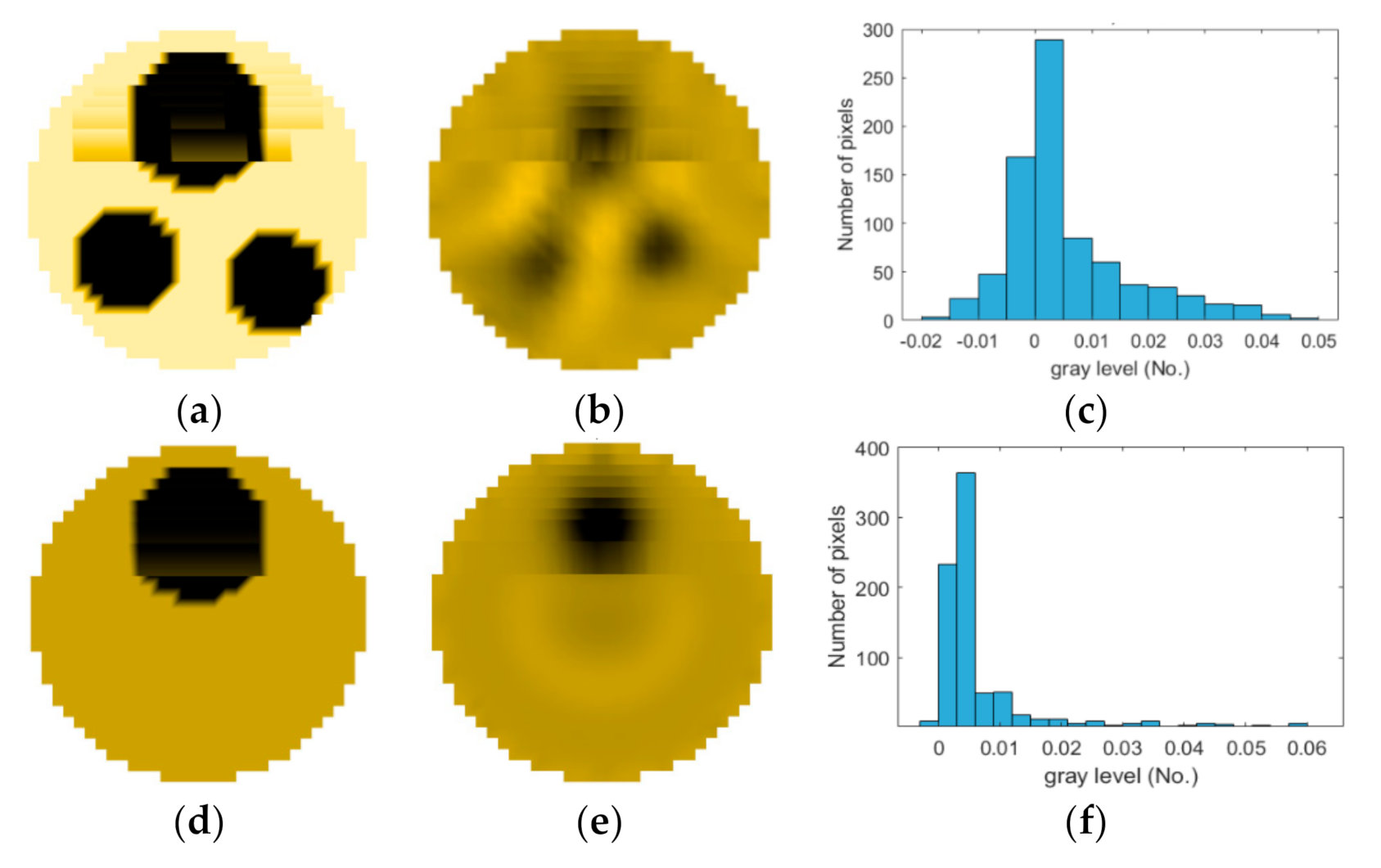
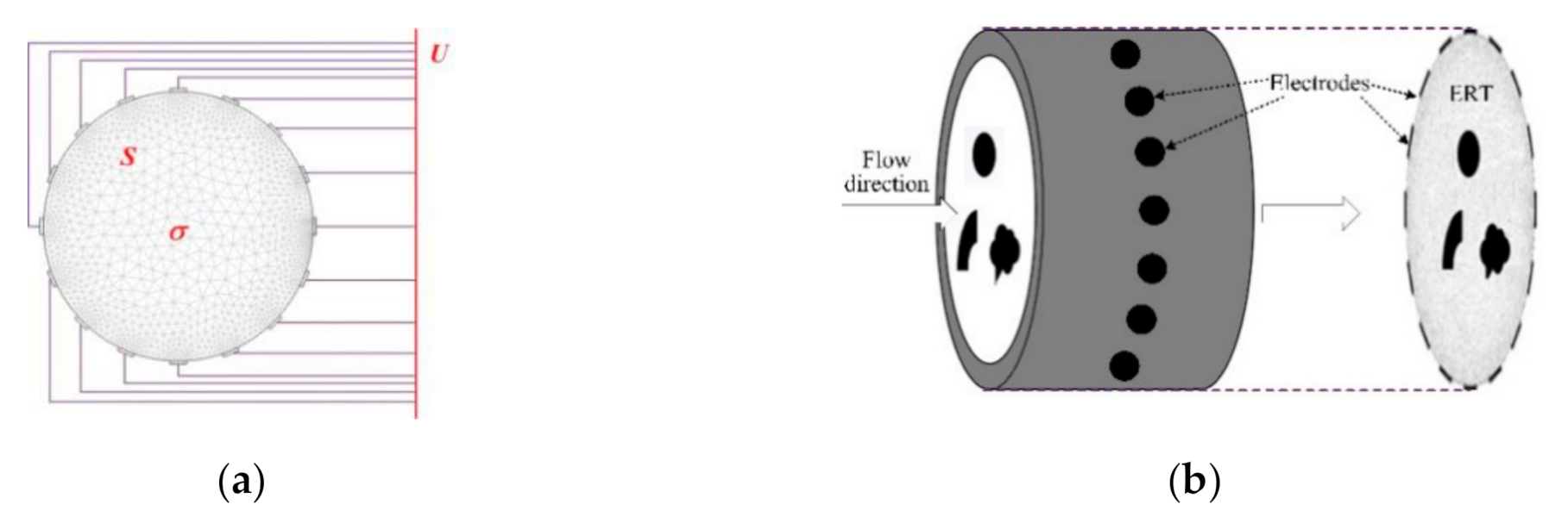
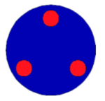
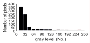
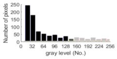
Figure 2a,d simulates two types of solid–liquid objects, (b) and (e) are their respective ERT images, and (c) and (f) are their statistical histograms related to all grey distributions of the pixels, where each bar along with the horizontal and vertical axis refer to the grey level interval and pixel number, respectively. These solid-phase and liquid-phase objects in (a) have a clear boundary, and these solid objects (in black) can be found in the related ERT image, as shown in (b). Any ERT-based CF method can correctly estimate the CF value with small error. However, when partial solid objects (e.g., two small circles in (a)) are dissolved or mixed into liquid-phase objects (see (d)), the ERT image cannot find them (see (e)) and the CF estimation may generate a large error. In particular, the statistical histogram (c) is more difficult to partition to two clusters than (f), since the latter has a more centralized peak whereas two separated peaks relative to solid and liquid objects are desired. Furthermore, any ERT image inevitably contains artifacts that cannot correctly be estimated by the existing method when computing the CF value. Consequently, the pixels that respond to the mixtures and artifacts make the real CF value estimation difficult to correctly estimate.
To solve the above problems, we first used the
f-FCM algorithm to partition all pixels in any ERT image into three clusters: solid, liquid, and their mixtures or artifacts. In the
f-FCM algorithm, all
n pixels are projected into
L grades of grey levels and represented as the discrete set:
Let
H(
l) be the number of pixels at the
l-th grey level,
l = 1, 2,…,
L, then the objective function of the
f-FCM algorithm is
where
uil is the membership degree of the
lth grey level to
ith cluster,
I = 1, 2, 3;
c is taken as 3, which refers to the partitioned number of clusters; and
m is a weighting exponent, and is often taken as 1.5, if no other information is available.
f-FCM updates cluster center and membership function as follows:
where
k is iteration times, and
The algorithm stops if the total residual error ||∑(uil(k+1) − uil (k))|| is smaller than a specified value ε, or k reaches a maximum number of iterations. In this paper, the termination residual error and the maximum number of iterations were taken as 10−5 and 100, respectively.
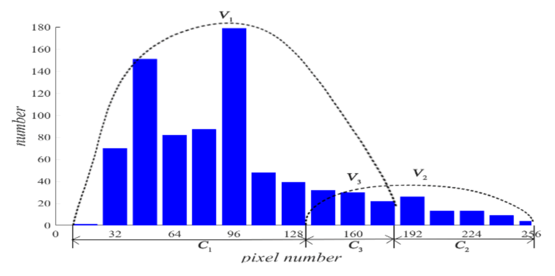
Assume that all pixels in
G in an ERT image is partitioned by the
f-FCM algorithm to three clusters
C1,
C2, and
C3 that have respective centers
v1,
v2, and
v3, and respective numbers of pixels
n1,
n2, and
n3 (see
Figure 3). Let
D1(
j) and
D2(
j) be the distance of the
jth pixel in
C3 to clustering prototypes
v1 and
v2, respectively. Following common practice, first, the values of
D1(
j) and
D2(
j) reflect the respective possibility that the
jth pixel belongs to
C1 and
C2. Closer distance to a center a pixel has, and larger possibility the pixel belongs to the cluster. Second, these pixels in
C3 result from artifacts or mixtures in
C1 and
C2, and the ratio that these pixels in
C3 belong to
C1 and
C2 is assumed to be directly proportional to the values of
n1 and
n2, respectively.
According to the following twin-weighted rule, all pixels in
C3 are partitioned to
C1 and
C2,
where
num(1) and
num(2) are the number of pixels that are individually assigned to
C1 and
C2, and
The number of 1 in Equation (11) aims to prevent the value of
r1 and
r2 being overlarge. Consequently, the CF values in the solid and liquid phases are individually estimated as
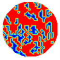
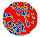
Table 1 shows a group of ERT images by LBP, and evaluation results of
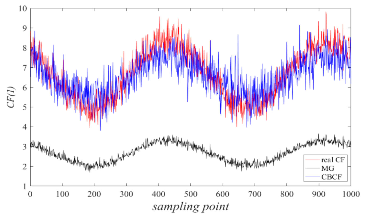
CF(1) by the MG method, where
CF(1) with respect to the solid component fraction is taken from 10% to 40% increasingly, and the conductivity of objects and backgrounds are set to 0.01 and 10, respectively. Here the bars in red, green, and blue in these histograms refer to the three partitioned clusters by
f-FCM, respectively.
From these various models, the obtained accuracy by Equation (12) was higher than the MG method in all four models, whereas the MG method tends to underestimate the real value in most cases. When the ERT image contains artifacts, MG causes a large error, but Equation (12) is affected to a small extent. These results show the correction of Equation (12) when the detected solid-phase objects can be distinguished by ERT. Therefore, the CF estimation by Equation (12) does not need other prior information, and thus is easily realized and comprehensive.
3.2. Computation on Undistinguishable Objects by Prior Information Inquiry
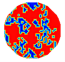
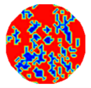
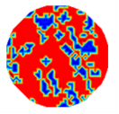
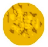
If any solid object size is very small, ERT cannot find the object at all, so Equation (12) must be inaccurate. Let five simulating solid–liquid flow patterns have the same value of
CF(1), 0.360, but different solid object sizes.
Table 2 shows the ERT images, partitioned clusters by
f-FCM, and computed values of
CF(1) by Equation (12) on the five patterns, respectively. As solid object size gradually decreases so that ERT cannot distinguish most solid objects, when using
f-FCM, these undistinguishable objects are incorrectly partitioned to
C2 or
C3 and make the estimated
CF(1) generate a very large error. Therefore,
CF (1) in Equation (12) must be corrected and recomputed.
Note that these pixels in
C1 are very different from those in
C2 or
C3, and the former basically consists of solid-phase objects whereas the latter may contain partial solid-phase objects that ERT cannot distinguish. Hence, we estimated
CF(1) by two steps. First, all pixels in the ERT image are clustered by
f-FCM to construct a set that is still denoted as
C1 with the number of pixels
n1, which responds to these distinguishable solid-phase objects by ERT. Then, all undistinguishable objects that are contained in the rest of the pixels are estimated by a grey index:
where both values of
sij and
ui are available in any ERT process, and Φ consists of all pixels in the detected field with the number of pixels
n. The number ‘
n’ in Equation (13) aims to normalize the value of
σ(
Cu) to each pixel. Generally, in dredging engineering, the conductivity of liquid-phase pixels (e.g., seawater) are known in advance. Furthermore, assuming that actual solid-phase objects in Φ consist of
ns pixels, if
C1 is determined by
f-FCM and
ns is fixed, (
ns–n1) is just the number of pixels that construct undistinguishable objects. Generally, the value of
σ(
Cu) is nearly unchangeable regardless of how the (
ns–n1) pixels are distributed, as explained below.
Table 3 shows a group of randomly distributed pixels that respond to undistinguishable objects, where the values of
ns/
n are always taken as 0.40, but the value of
n1/
n in all models was selected as nearly 0.30. Therefore, the value of
σ(
Cu) is approximately unchangeable. In fact, according to the Ohm theorem [
21], the area and the length of the method from injecting to measuring electrodes is nearly unchangeable under various pixel distributions if the value of (
n1–
ns) is fixed. The conclusion was verified by our previous work [
28]. Consequently, according to the value of
σ(
Cu) and the determined pixels in
C1 by
f-FCM, the interrelation between (
ns–n1) and
σ(
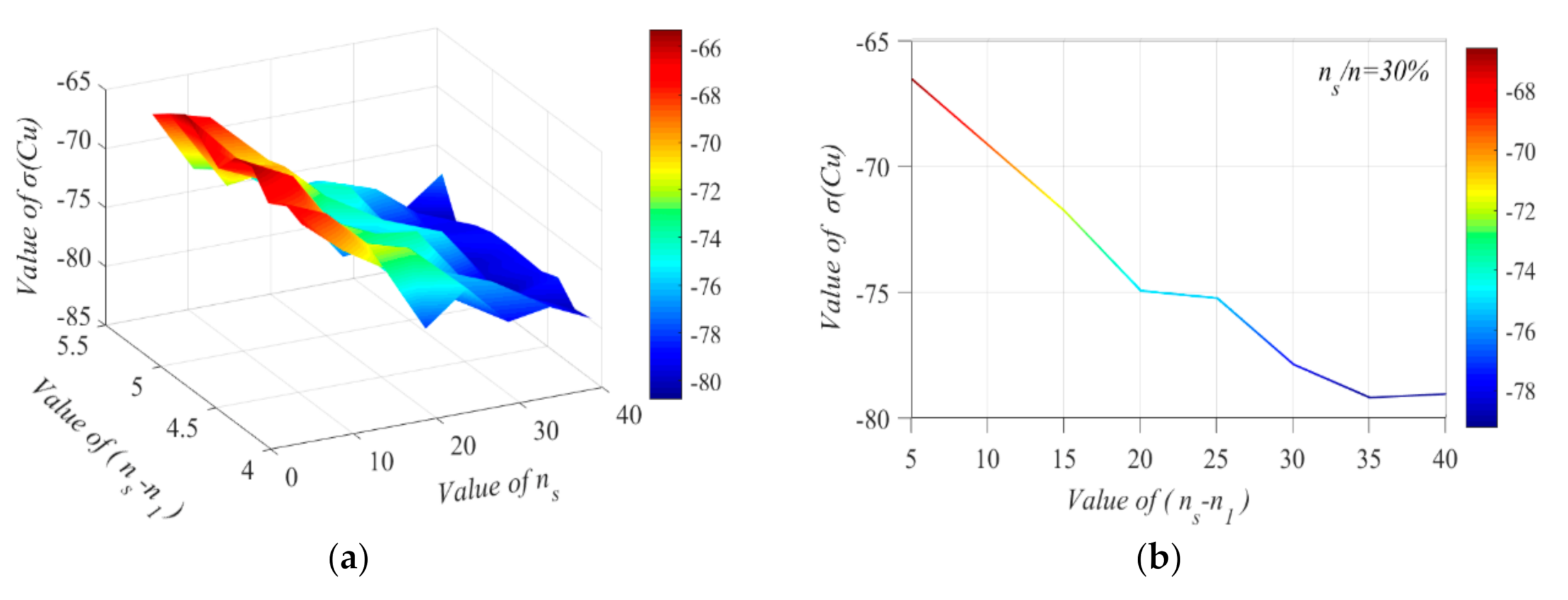
Cu) can be determined prior.
Figure 4a shows the varied curve of
σ(
Cu) as the two relative variables of
n1 and (
ns–n1) are changed. It can be observed that (
ns–n1) is tightly relative to the value of
σ(
Cu). Alternatively,
Figure 4b shows the changing trend of (
ns–n1) as
σ(
Cu) increases when
n1/
n = 0.3.
Table 4 shows the correlation between
n1,
σ(
Cu), and (
ns–n1). It provides a way to estimate the value of (
ns–n1) when
n1 and
σ(
Cu) are known. Consequently, after determining the value of
n1 by
f-FCM and the value of (
ns–n1) by
σ(
Cu), the value of
CF(1) can be computed as:
According to Equation (14), the proposed CF estimation method is presented in Algorithm 1:
| Algorithm 1. The proposed CF estimation method. |
Input: Boundary measurements and sensitivity matrix S
Output: CF(1)- (1)
Image the detected field by ERT; - (2)
Cluster all pixels by f-FCM; - (3)
Determine C1 and n1; - (4)
Compute σ(Cu) by Equation (13); - (5)
Inquiry (ns–n1) by prior knowledge based on σ(Cu); - (6)
Compute CF(1) by Equation (14).
|
Hereafter, we call the cluster-based CF estimation CBCF.


 background
  artifacts
  object