Automatic Calibration of a Two-Axis Rotary Table for 3D Scanning Purposes


Abstract
:1. Introduction
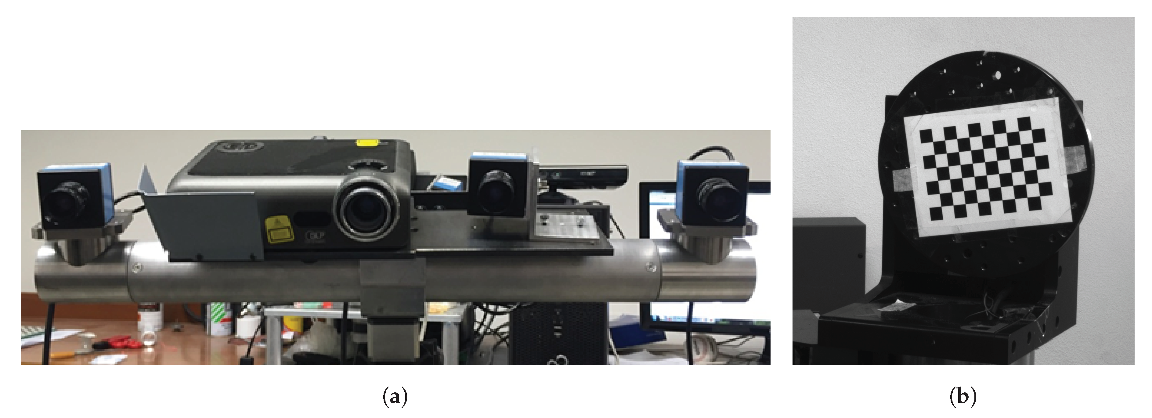
2. Materials
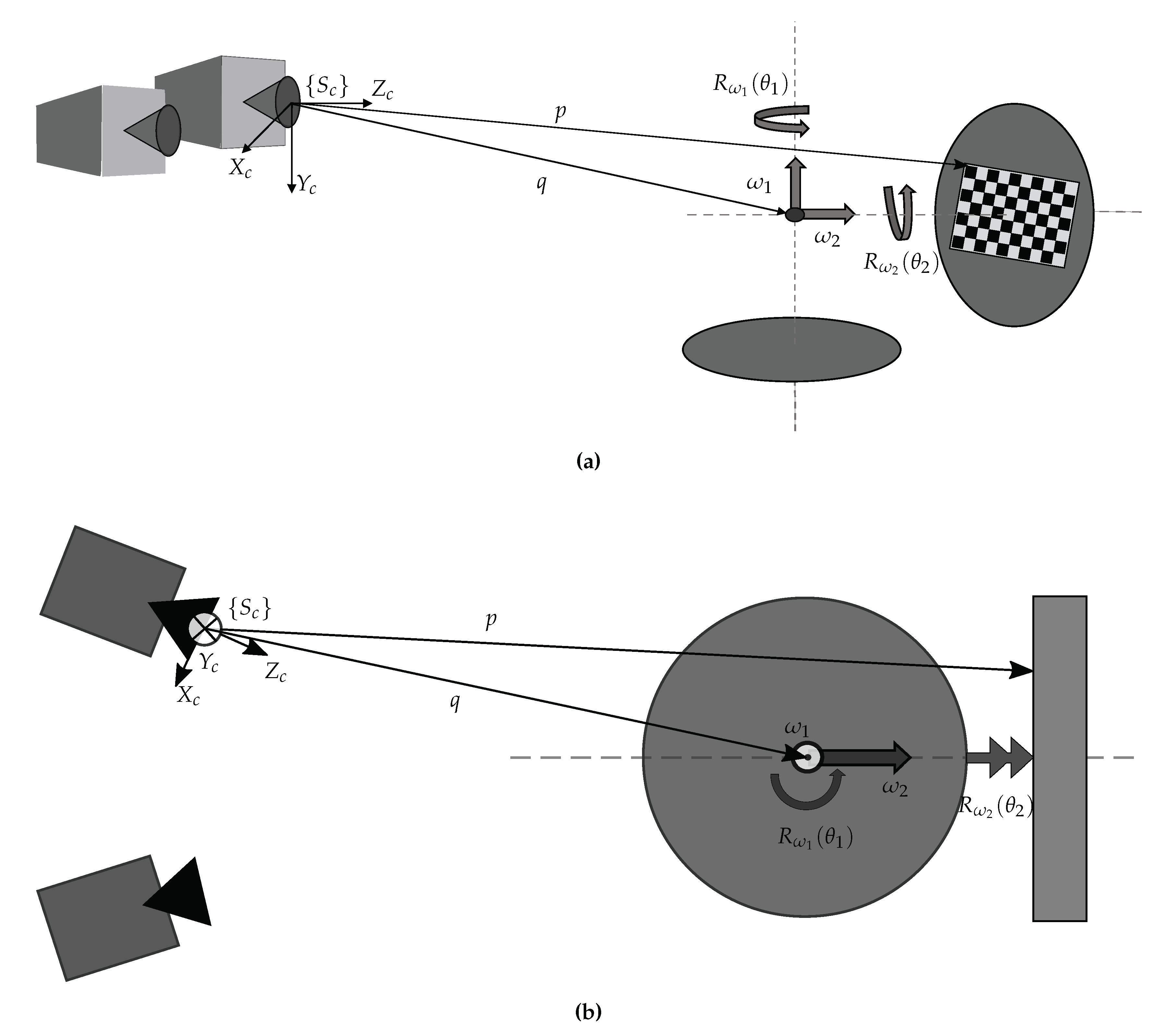
3. Calibration Approach
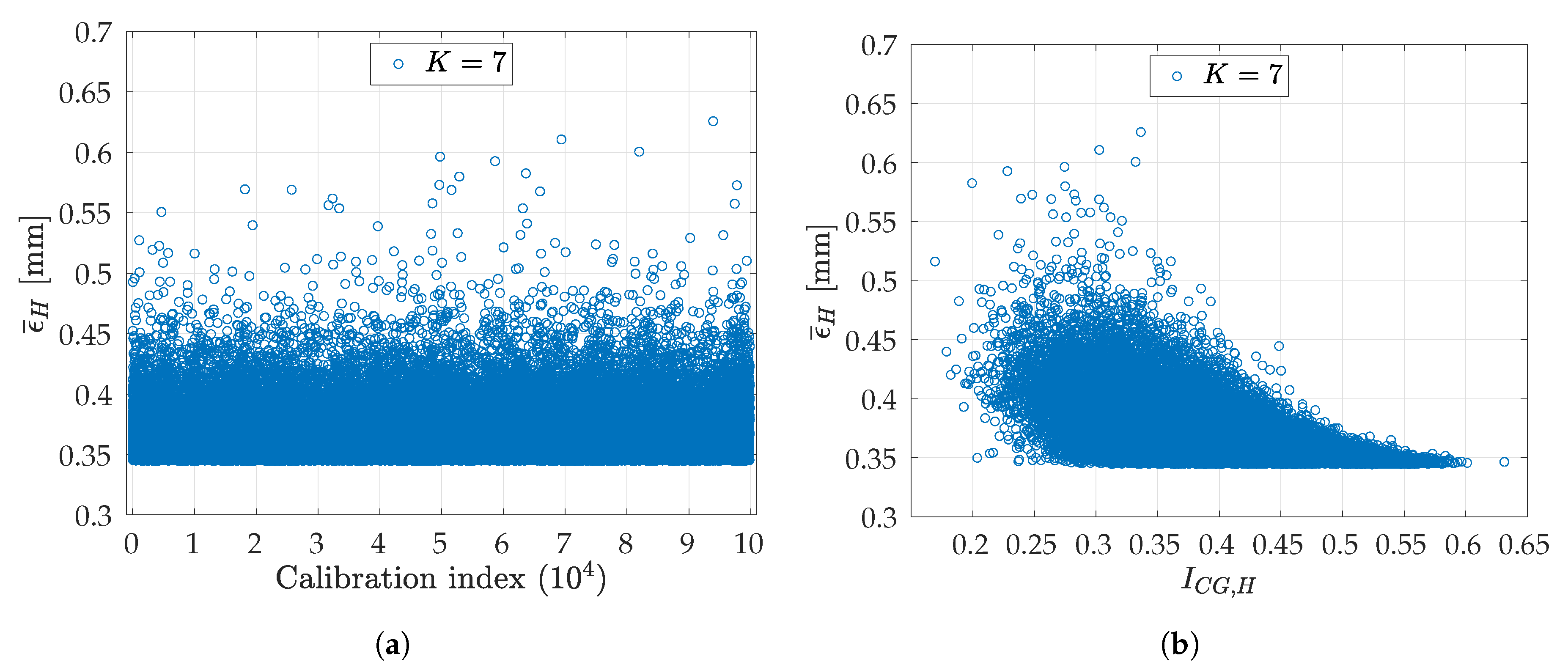
4. Influence of the Number of Calibration Images
4.1. Data Set Definition
- ;
- , where ;
- , where ;
- , where ;
- is a set of indices i, where , that denotes the pairs of angular positions , , of the subset of images to calibrate with;
- , , is the size of H, i.e., the number of images considered;
- .
4.2. Error Metric Definition
4.3. Methods Comparison
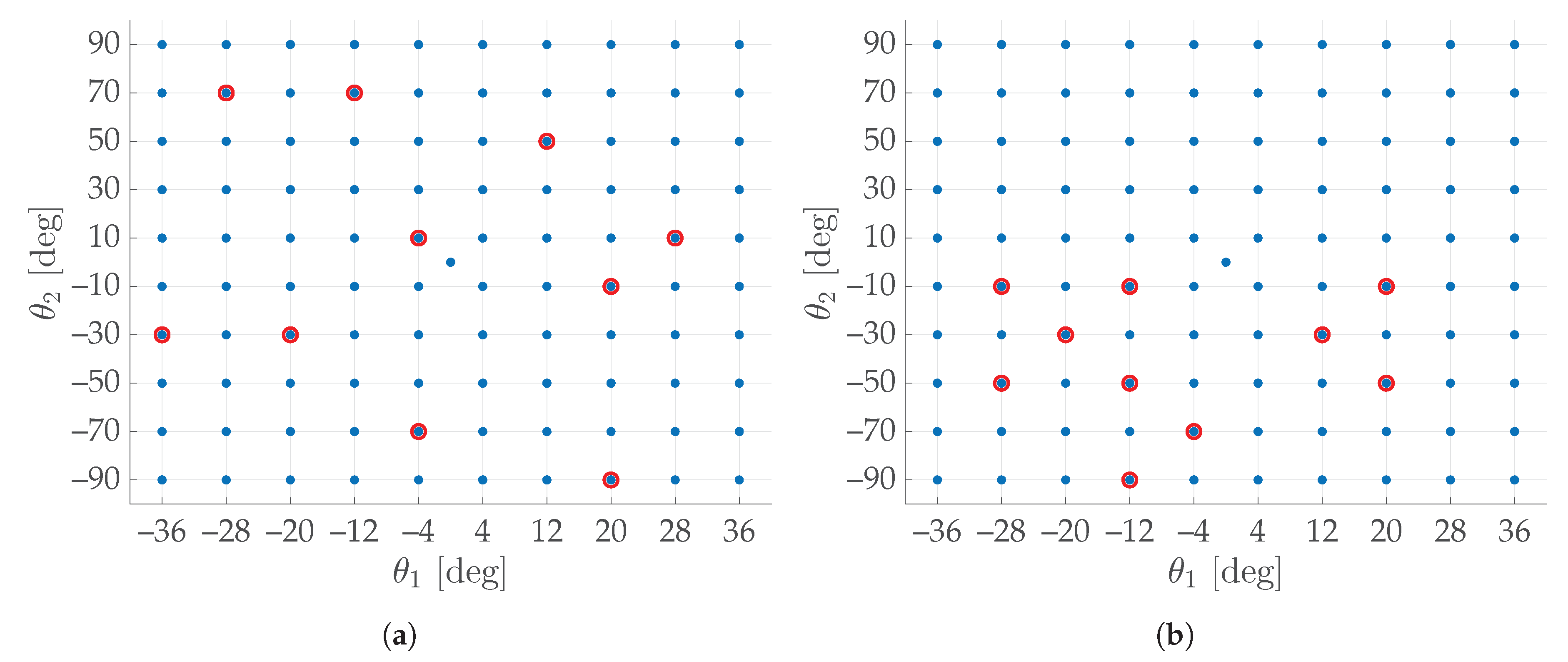
5. Optimal Calibration Set
5.1. Complete Graph Index
- is the set of vertices (normalized angular positions);
- is the set of edges;
- is a graph;
- ;
- is the weight function;
5.2. Index-Based Analysis and Experimental Results
6. Conclusions
Author Contributions
Funding
Acknowledgments
Conflicts of Interest
Appendix A
- Settings;
- Turntable Control;
- Image Acquisition;
- Stereo-Camera Calibration;
- Turntable Calibration;
- Error Analysis.
- activate/deactivate the motors connected to the shield via Arduino and to specify its serial port;
- activate/deactivate the camera(s) connected to the computer, adjusting several parameters such as exposure, image format, image resolution, and frame rate.

- the square dimensions of the checkerboard;
- the desired image format;
- the target poses of the turntable, in the form of pairs of angular positions , , where is the number of acquisitions, with respect to the reference pose .
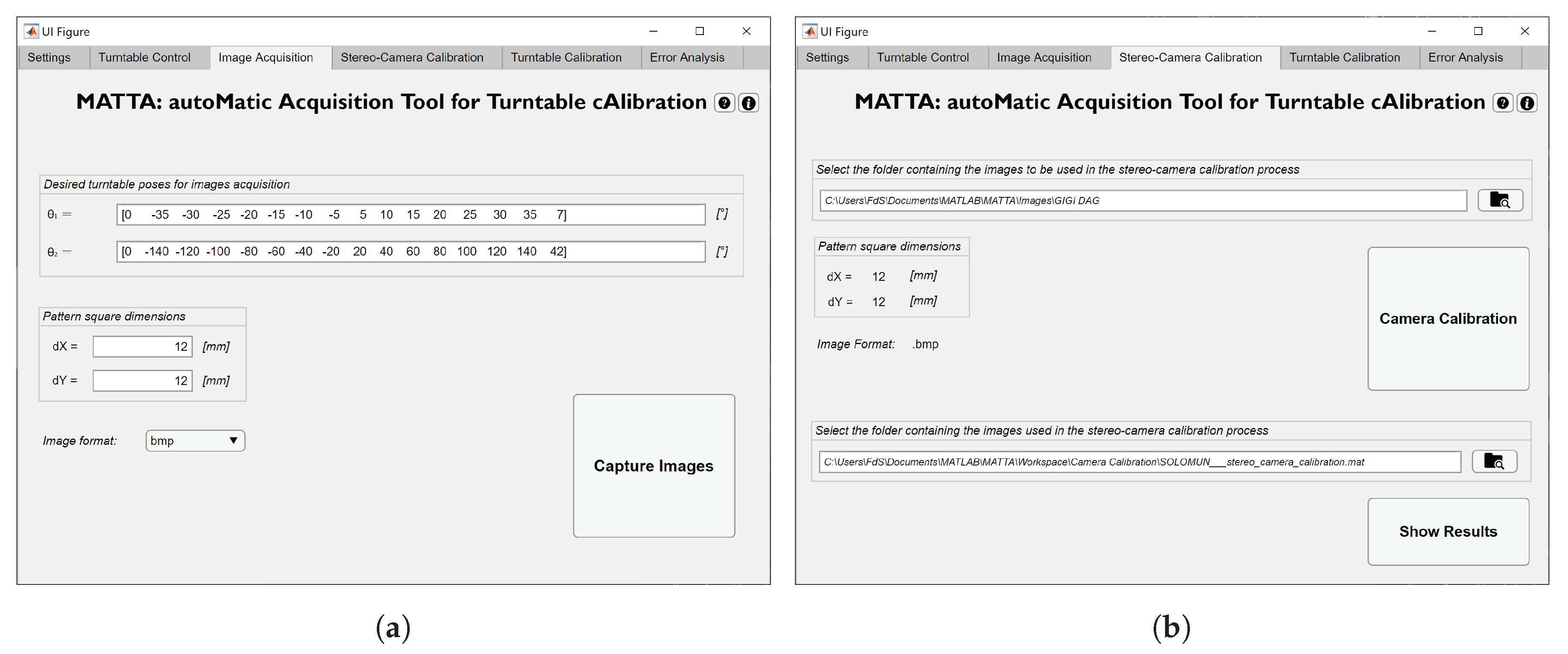
- a stereo-camera calibration file previously generated in the Stereo-Camera Calibration tab;
- a folder of images previously acquired with the aid of the Image Acquisition tab. The GUI fills the Calibration set panel with a number of checkboxes equal to the number of stereo-pair images contained in the specified folder, i.e., . By means of the checkboxes, the user is able to select the K stereo-pair images to be used in the calibration procedure, thus constituting the desired subset H; alternatively, the entire set of images is used by default.


References
- Gorthi, S.; Rastogi, P. Fringe projection techniques: Whither we are? Opt. Lasers Eng. 2010, 48, 133–140. [Google Scholar] [CrossRef] [Green Version]
- Bernardini, F.; Rushmeier, H. The 3D Model Acquisition Pipeline. Comput. Graph. Forum 2002, 21, 149–172. [Google Scholar] [CrossRef]
- Barone, S.; Paoli, A.; Razionale, A.V. Three-dimensional point cloud alignment detecting fiducial markers by structured light stereo imaging. Mach. Vis. Appl. 2012, 23, 217–229. [Google Scholar] [CrossRef]
- Barone, S.; Paoli, A.; Razionale, A. Computer-aided modelling of three-dimensional maxillofacial tissues through multi-modal imaging. Proc. Inst. Mech. Eng. Part H J. Eng. Med. 2013, 227, 89–104. [Google Scholar] [CrossRef] [PubMed]
- Ye, J.; Xia, G.; Liu, F.; Cheng, Q. 3D reconstruction of line-structured light based on binocular vision calibration rotary axis. Appl. Opt. 2020, 59, 8272–8278. [Google Scholar] [CrossRef] [PubMed]
- Ahmadabadian, A.; Yazdan, R.; Karami, A.; Moradi, M.; Ghorbani, F. Clustering and selecting vantage images in a low-cost system for 3D reconstruction of texture-less objects. Measurement 2017, 99, 185–191. [Google Scholar] [CrossRef]
- Sun, J.; Zhang, Z.; Zhang, J. Reconstructing normal section profiles of 3D revolving structures via pose-unconstrained multi-line structured-light vision. IEEE Trans. Instrum. Meas. 2020, 70, 1. [Google Scholar] [CrossRef]
- Wang, C.; Zhou, X.; Fei, Z.; Gao, X.; Jin, R. A three dimensional point cloud registration method based on rotation matrix eigenvalue. In Society of Photo-Optical Instrumentation Engineers (SPIE) Conference Series; SPIE: Bellingham, WA, USA, 2017; Volume 10410, p. 1041014. Available online: https://spie.org/Publications/Proceedings/Paper/10.1117/12.2276849 (accessed on 9 December 2020).
- Dai, M.; Chen, L.; Yang, F.; He, X. Calibration of revolution axis for 360 deg surface measurement. Appl. Opt. 2013, 52, 5440–5448. [Google Scholar] [CrossRef]
- Gonzalez-Barbosa, J.J.; Rico-Espino, J.G.; Gómez-Loenzo, R.A.; Jiménez-Hernández, H.; Razo, M.; Gonzalez-Barbosa, R. Accurate 3D Reconstruction using a Turntable-based and Telecentric Vision. Automatika 2015, 56, 508–521. [Google Scholar] [CrossRef] [Green Version]
- Abdel-Aziz, Y.I.; Karara, H.M. Direct linear transformation from comparator coordinates into object space coordinates in close-range photogrammetry. Photogramm. Eng. Remote Sens. 2015, 81, 103–107. [Google Scholar] [CrossRef]
- Frugers, O.D.; Toscani, G. The calibration problem for stereo. In Proceedings of the CVPR ’86, Miami Beach, FL, USA, 22–26 June 1986; IEEE: Piscataway, NJ, USA, 1986; pp. 15–20. [Google Scholar]
- Brown, D. Close-range camera calibration. Photogramm. Eng. Remote. Sens. 1971, 37, 855–866. [Google Scholar]
- Haralick, R.M.; Shapiro, L.G. Computer and Robot Vision, 2nd ed.; Addison–Wesley: Reading, MA, USA, 1993. [Google Scholar]
- Nomura, Y.; Sagara, M.; Naruse, H.; Ide, A. Simple calibration algorithm for high-distortion lens camera. IEEE Trans. Pattern Anal. Mach. Intell. 1992, 14, 1095–1099. [Google Scholar] [CrossRef]
- Weng, J.; Cohen, P.; Herniou, M. Camera calibration with distortion models and accuracy evaluation. IEEE Trans. Pattern Anal. Mach. Intell. 1992, 14, 965–980. [Google Scholar] [CrossRef] [Green Version]
- Barone, S.; Neri, P.; Paoli, A.; Razionale, A. Flexible calibration of a stereo vision system by active display. In Procedia Manifacturing; Elsevier B.V.: Amsterdam, The Netherlands, 2019; Volume 38, pp. 564–572. [Google Scholar]
- Barone, S.; Neri, P.; Paoli, A.; Razionale, A. 3D acquisition and stereo-camera calibration by active devices: A unique structured light encoding framework. Opt. Lasers Eng. 2020, 127, 105989. [Google Scholar] [CrossRef]
- Barone, S.; Neri, P.; Paoli, A.; Razionale, A. Structured light stereo catadioptric scanner based on a spherical mirror. Opt. Lasers Eng. 2018, 107, 1–12. [Google Scholar] [CrossRef]
- Agrawal, A.; Taguchi, Y.; Ramalingam, S. Analytical Forward Projection for Axial Non-central Dioptric and Catadioptric Cameras. In Computer Vision—ECCV 2010; Daniilidis, K., Maragos, P., Paragios, N., Eds.; Springer: Berlin/Heidelberg, Germany, 2010; pp. 129–143. [Google Scholar]
- Baker, S.; Nayar, S. A theory of single-viewpoint catadioptric image formation. Int. J. Comput. Vis. 1999, 35, 175–196. [Google Scholar] [CrossRef]
- Barone, S.; Carulli, M.; Neri, P.; Paoli, A.; Razionale, A.V. An omnidirectional vision sensor based on a spherical mirror catadioptric system. Sensors 2018, 18, 408. [Google Scholar] [CrossRef] [Green Version]
- Mülayim, A.; Yemez, Y.; Schmitt, F.; Atalay, V. Rotation axis extraction of a turn table viewed by a fixed camera. In Vision, Modeling and Visualisation ’99; IOS Press: Amsterdam, The Netherlands, 1999; pp. 35–42. [Google Scholar]
- Li, J.; Chen, M.; Jin, X.; Chen, Y.; Dai, Z.; Ou, Z.; Tang, Q. Calibration of a multiple axes 3-D laser scanning system consisting of robot, portable scanner and turntable. Optik 2011, 122, 324–329. [Google Scholar] [CrossRef]
- Xu, Y.; Yang, Q.; Huai, J. Calibration of the axis of the turntable in 4-axis laser measuring system and registration of multi-view. Chin. J. Lasers 2005, 32, 659–662. [Google Scholar]
- Bi, C.; Hao, X.; Liu, M.; Fang, J. Study on calibration method of rotary axis based on vision measurement. Infrared Laser Eng. 2020, 49. [Google Scholar] [CrossRef]
- Langming, Z.; Xiaohu, Z.; Banglei, G. A flexible method for multi-view point clouds alignment of small-size object. Measurement 2014, 58, 115–129. [Google Scholar] [CrossRef]
- Ye, Y.; Song, Z. An accurate 3D point cloud registration approach for the turntable-based 3D scanning system. In Proceedings of the 2015 IEEE International Conference on Information and Automation (ICIA), Kunming, China, 8–10 August 2015; pp. 982–986. [Google Scholar]
- Chen, P.; Dai, M.; Chen, K.; Zhang, Z. Rotation axis calibration of a turntable using constrained global optimization. Optik 2014, 125, 4831–4836. [Google Scholar] [CrossRef]
- Bisogni, L.; Pettinari, M.; Mollaiyan, R. MATTA: AutoMatic Acquisition Tool for Turntable cAlibration. 2020. Available online: https://www.mathworks.com/matlabcentral/fileexchange/84124-matta-automatic-acquisition-tool-for-turntable-calibration?s_tid=srchtitle (accessed on 10 December 2020).
- MATLAB. 9.8.0.1451342 (R2020a); The MathWorks Inc.: Natick, MA, USA, 2020; Available online: https://www.mathworks.com/ (accessed on 9 December 2020).
- Bouguet, J.Y. Camera Calibration Toolbox for MATLAB. 2015. Available online: http://www.vision.caltech.edu/bouguetj/calib_doc/ (accessed on 9 December 2020).


| Combination | Circles method | Proposed method | ||
|---|---|---|---|---|
| H | [mm] | [mm] | [mm] | [mm] |
| 1.6956 | 0.1488 | 0.3579 | 0.1758 | |
| 0.8038 | 0.2310 | 0.3414 | 0.1711 | |
| 0.5283 | 0.1833 | 0.3352 | 0.1678 | |
| K | [%] | ||
|---|---|---|---|
| 2 | 0.8958 | 0.3747 | 8.72 |
| 0.3643 | 5.73 | ||
| 0.3533 | 2.52 | ||
| 0.3490 | 1.28 | ||
| 4 | 0.7225 | 0.3469 | 0.67 |
| 7 | 0.6313 | 0.3466 | 0.58 |
| 46 | 0.4226 | 0.3445 | 0.02 |
Publisher’s Note: MDPI stays neutral with regard to jurisdictional claims in published maps and institutional affiliations. |
© 2020 by the authors. Licensee MDPI, Basel, Switzerland. This article is an open access article distributed under the terms and conditions of the Creative Commons Attribution (CC BY) license (http://creativecommons.org/licenses/by/4.0/).
Share and Cite
Bisogni, L.; Mollaiyan, R.; Pettinari, M.; Neri, P.; Gabiccini, M. Automatic Calibration of a Two-Axis Rotary Table for 3D Scanning Purposes. Sensors 2020, 20, 7107. https://doi.org/10.3390/s20247107
Bisogni L, Mollaiyan R, Pettinari M, Neri P, Gabiccini M. Automatic Calibration of a Two-Axis Rotary Table for 3D Scanning Purposes. Sensors. 2020; 20(24):7107. https://doi.org/10.3390/s20247107
Chicago/Turabian StyleBisogni, Livio, Ramtin Mollaiyan, Matteo Pettinari, Paolo Neri, and Marco Gabiccini. 2020. "Automatic Calibration of a Two-Axis Rotary Table for 3D Scanning Purposes" Sensors 20, no. 24: 7107. https://doi.org/10.3390/s20247107
APA StyleBisogni, L., Mollaiyan, R., Pettinari, M., Neri, P., & Gabiccini, M. (2020). Automatic Calibration of a Two-Axis Rotary Table for 3D Scanning Purposes. Sensors, 20(24), 7107. https://doi.org/10.3390/s20247107