Data-Driven Modeling of Smartphone-Based Electrochemiluminescence Sensor Data Using Artificial Intelligence

 , ,
, ,
Abstract
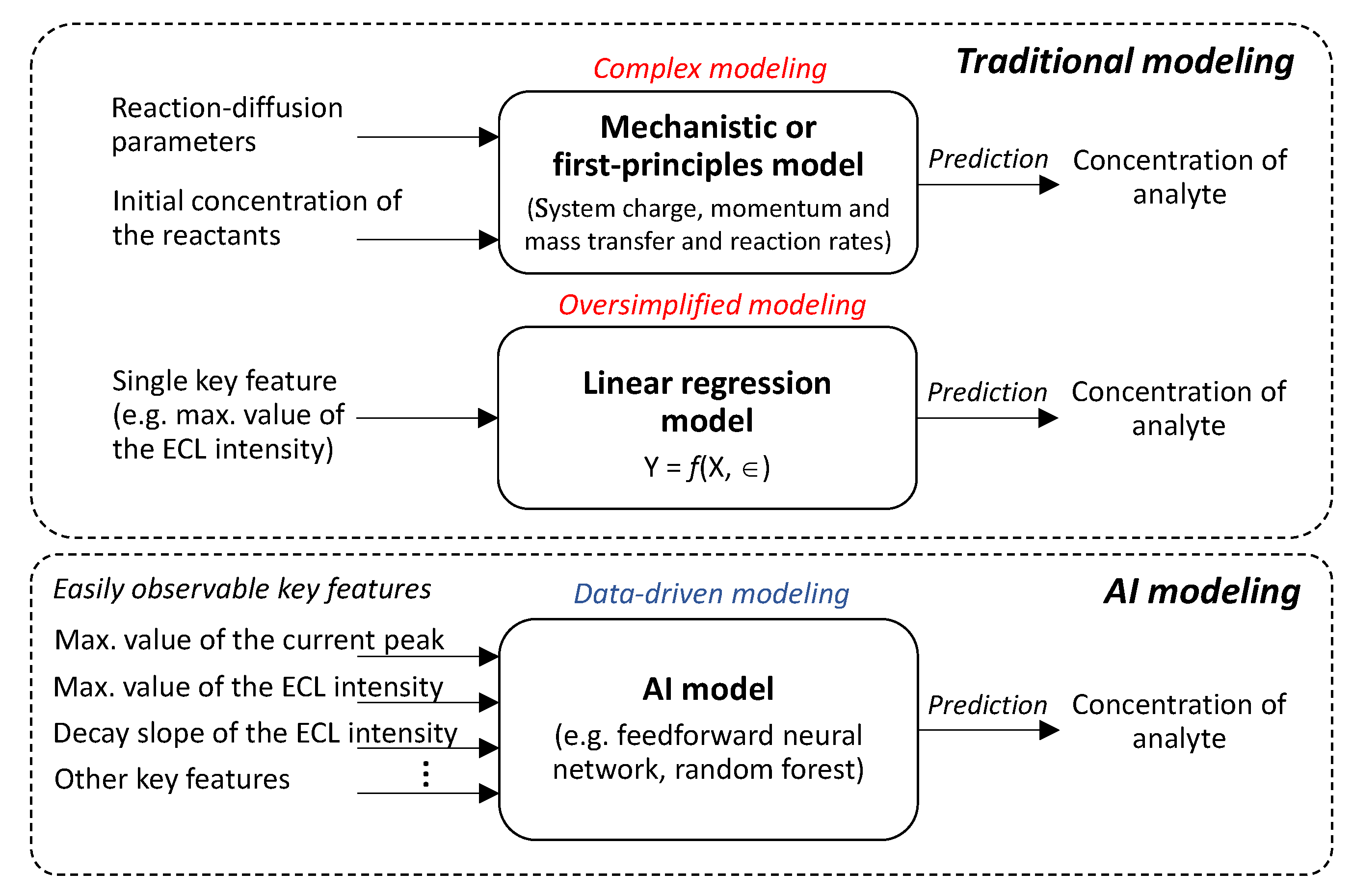
1. Introduction
2. Materials and Methods
2.1. Chemical and Reagents
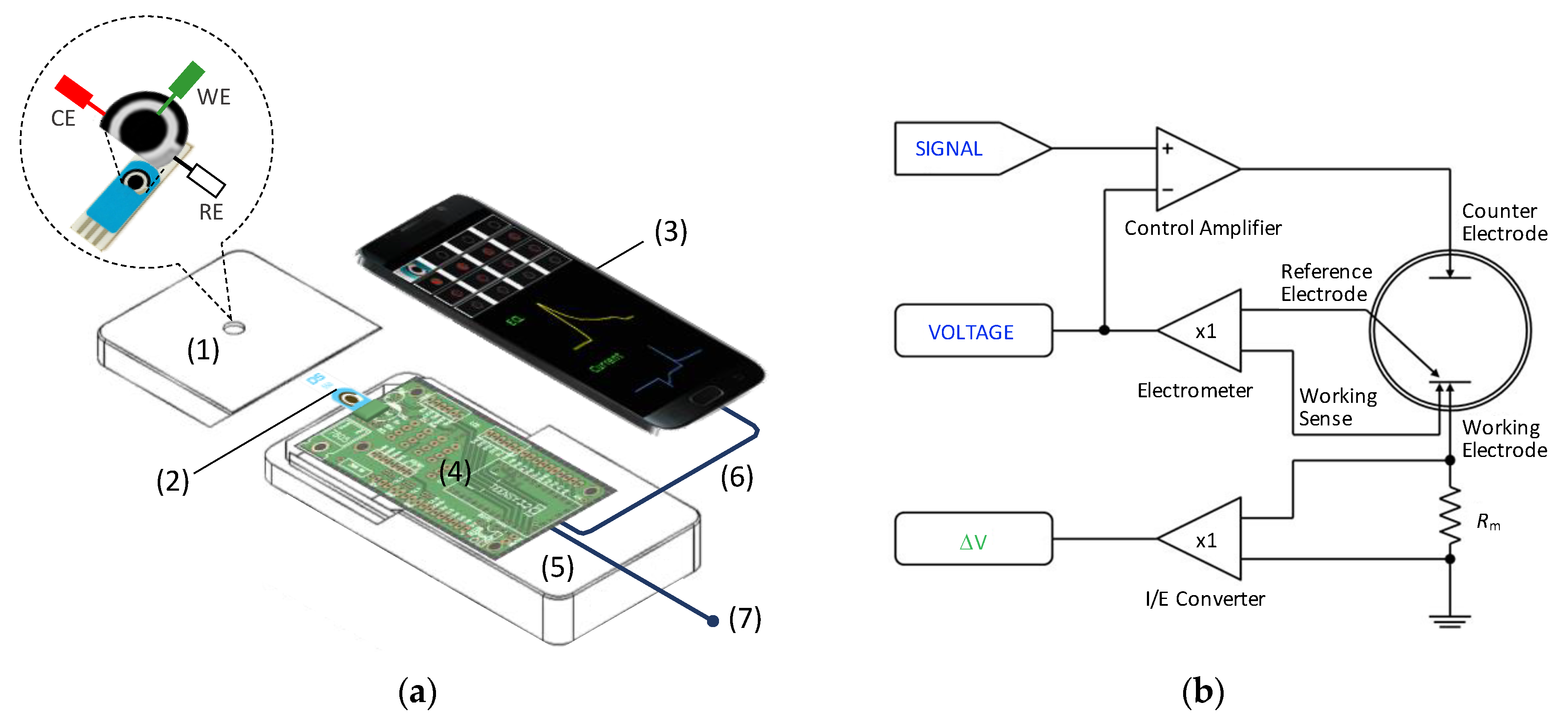
2.2. Sensor Apparatus and Electrodes
2.3. Assays
2.4. Electrochemical and ECL Experimental Data Generation
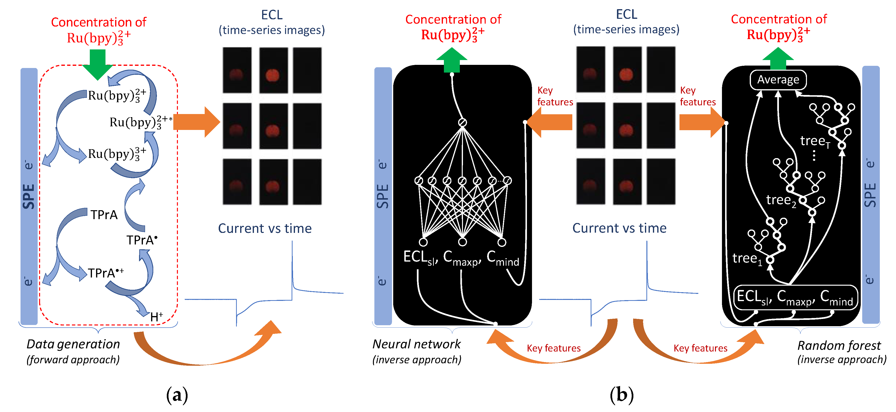
2.5. AI algorithms
2.5.1. Random Forest (RF)
2.5.2. Feedforward Neural Network (FNN)
3. Results and Discussion
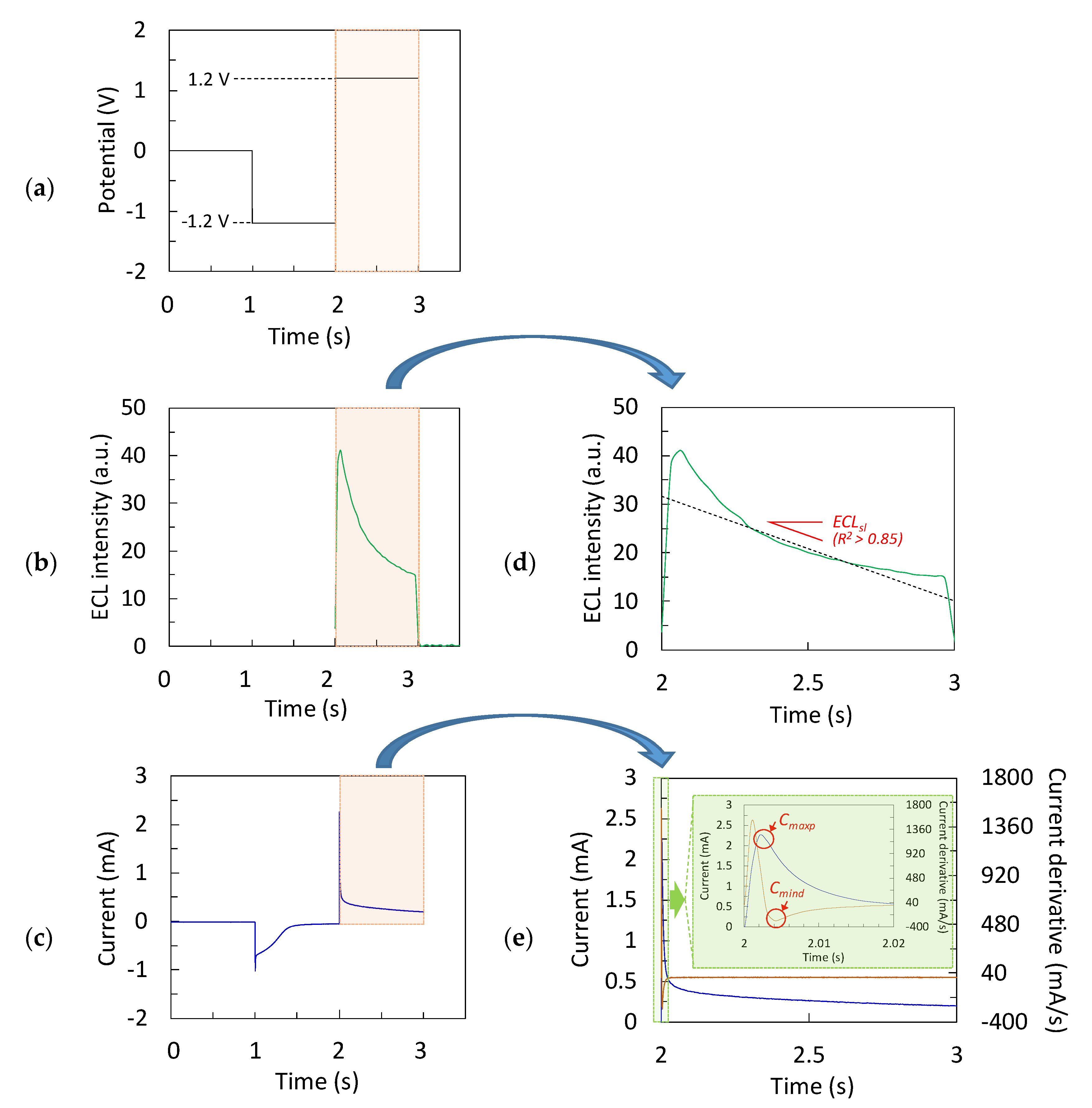
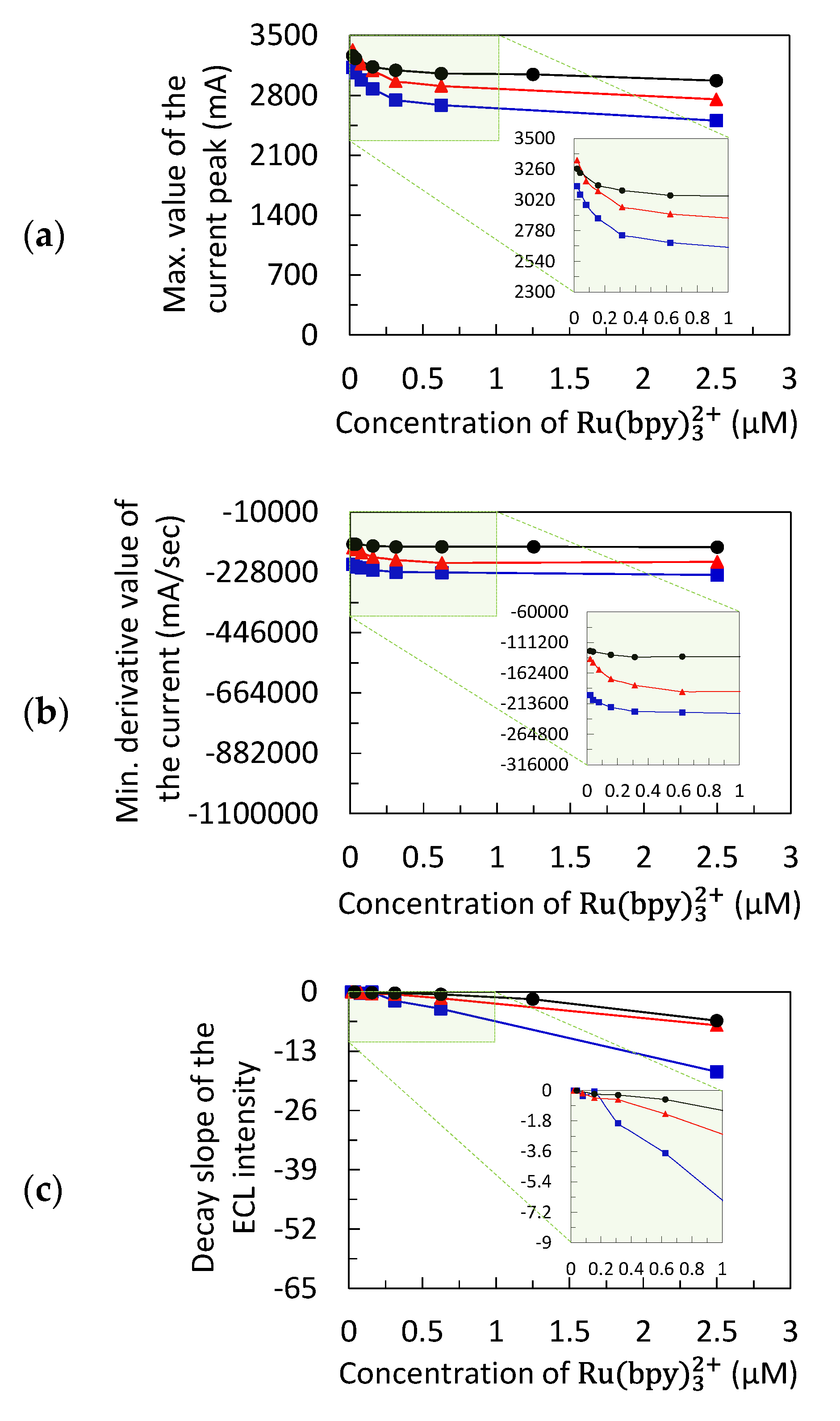
3.1. Chronoamperometric Data for Data-Driven Modeling
3.2. Data-Driven Model Calibration and Prediction of
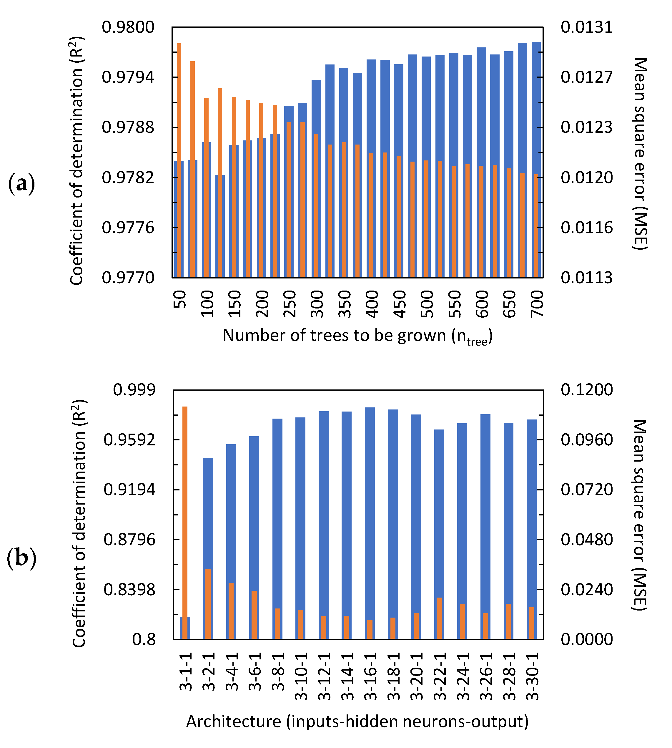
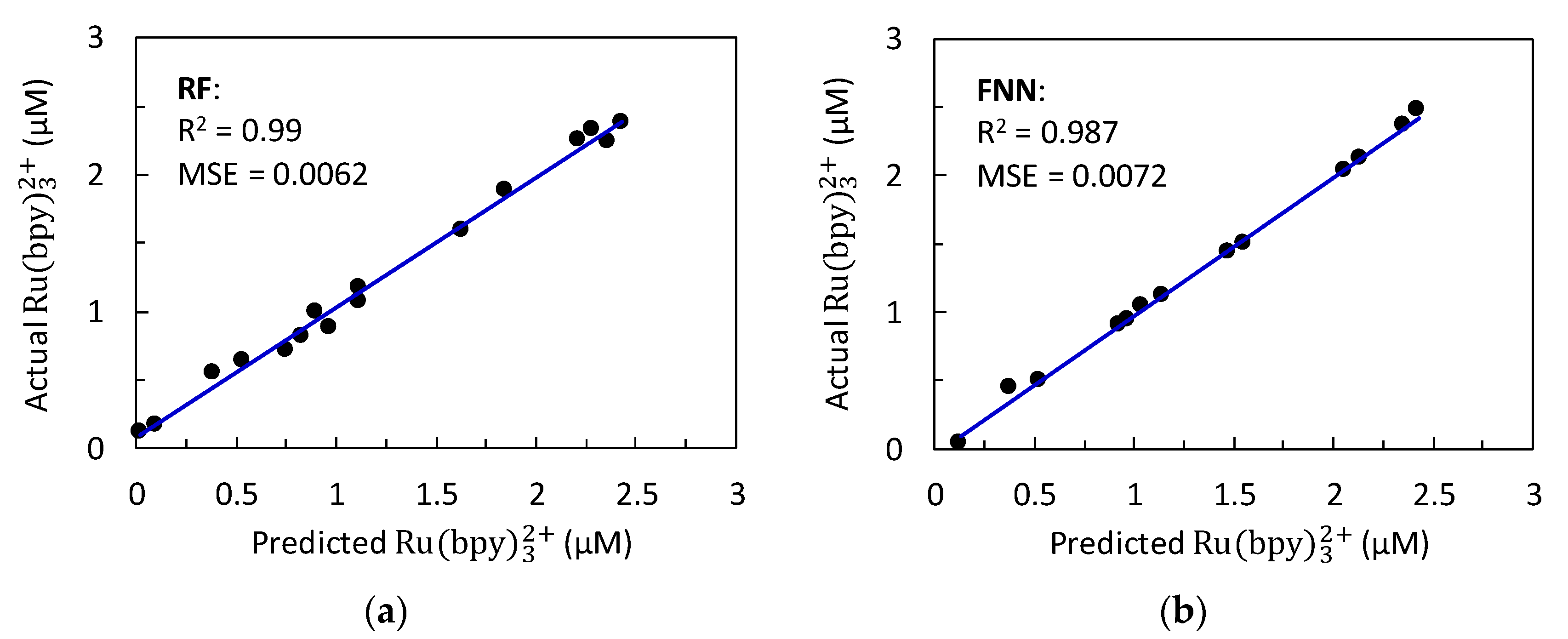
3.2.1. Random Forest (RF) Prediction Results
3.2.2. Feedforward Neural Network (FNN) Prediction Results
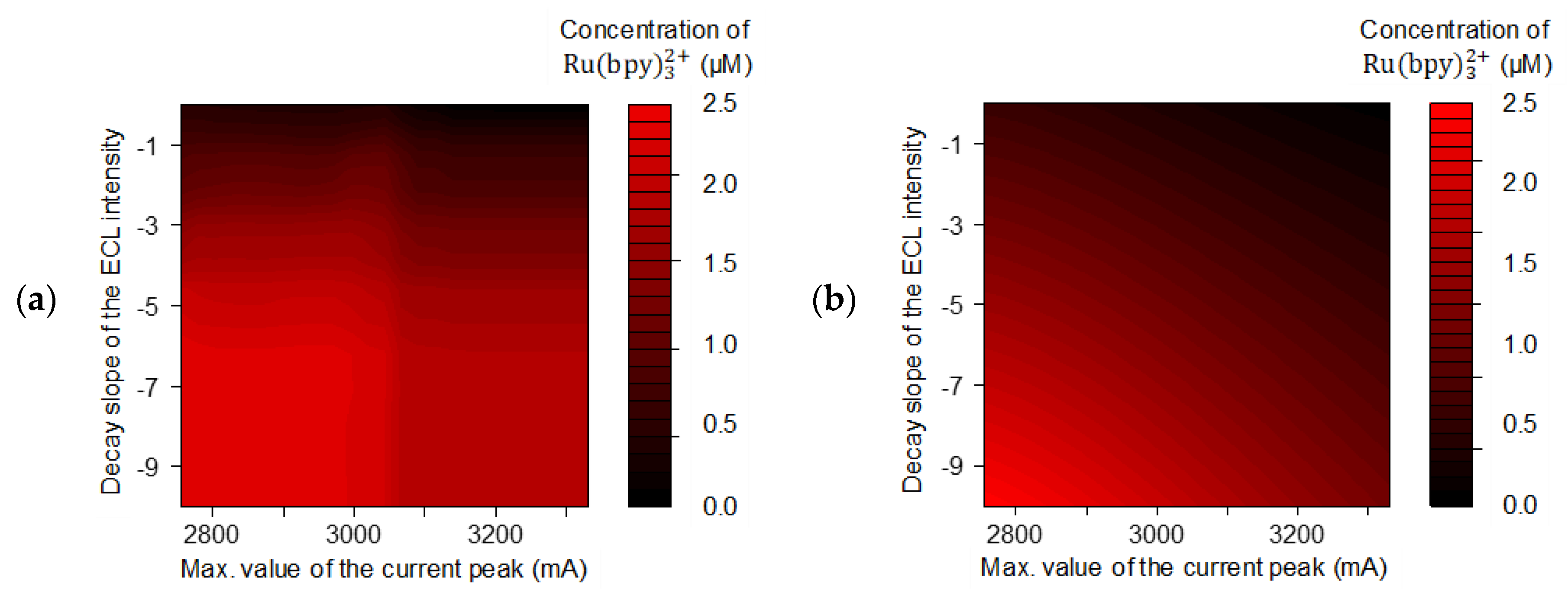
3.2.3. Visualizing Relationships between the Key Features and the Concentration of
4. Conclusions
Author Contributions
Funding
Conflicts of Interest
References
- Kwon, H.J.; Rivera, E.C.; Neto, M.R.C.; Marsh, D.; Swerdlow, J.J.; Summerscales, R.L.; Uppala, P.P.T. Development of smartphone-based ECL sensor for dopamine detection: Practical approaches. Res. Chem. 2020. accepted. [Google Scholar] [CrossRef]
- Zanut, A.; Fiorani, A.; Rebeccani, S.; Kesarkar, S.; Valenti, G. Electrochemiluminescence as emerging microscopy techniques. Anal. Bioanal. Chem. 2019, 411, 4375–4382. [Google Scholar] [CrossRef] [PubMed]
- Yao, Y.; Li, H.; Wang, D.; Liu, C.; Zhang, C. An electrochemiluminescence cloth-based biosensor with smartphone-based imaging for detection of lactate in saliva. Analyst 2017, 142, 3715–3724. [Google Scholar] [CrossRef] [PubMed]
- Li, S.; Zhang, D.; Liu, J.; Cheng, C.; Zhu, L.; Li, C.; Lu, Y.; Low, S.S.; Su, B.; Liu, Q. Electrochemiluminescence on smartphone with silica nanopores membrane modified electrodes for nitroaromatic explosives detection. Biosens. Bioelectron. 2019, 129, 284–291. [Google Scholar] [CrossRef] [PubMed]
- Li, S.; Lu, Y.; Liu, L.; Low, S.S.; Su, B.; Wu, J.; Zhu, L.; Li, C.; Liu, Q. Fingerprints mapping and biochemical sensing on smartphone by electrochemiluminescence. Sens. Actuators B Chem. 2019, 285, 34–41. [Google Scholar] [CrossRef]
- Danis, A.S.; Potts, K.P.; Perry, S.C.; Mauzeroll, J. Combined spectroelectrochemical and simulated insights into the electrogenerated chemiluminescence coreactant mechanism. Anal. Chem. 2018, 90, 7377–7382. [Google Scholar] [CrossRef]
- Danis, A.S.; Gordon, J.B.; Potts, K.P.; Stephens, L.I.; Perry, S.C.; Mauzeroll, J. Simultaneous electrochemical and emission monitoring of electrogenerated chemiluminescence through instrument hyphenation. Anal. Chem. 2019, 91, 2312–2318. [Google Scholar] [CrossRef]
- Dong, X.; Zhao, G.; Liu, L.; Li, X.; Wei, Q.; Cao, W. Ultrasensitive competitive method-based electrochemiluminescence immunosensor for diethylstilbestrol detection based on Ru (bpy)32+ as luminophor encapsulated in metal–organic frameworks UiO-67. Biosens. Bioelectron. 2018, 110, 201–206. [Google Scholar] [CrossRef]
- Liu, Z.; Qi, W.; Xu, G. Recent advances in electrochemiluminescence. Chem. Soc. Rev. 2015, 44, 3117–3142. [Google Scholar] [CrossRef]
- Zhang, J.; Arbault, S.; Sojic, N.; Jiang, D. Electrochemiluminescence imaging for bioanalysis. Annu. Rev. Anal. Chem. 2019, 12, 275–295. [Google Scholar] [CrossRef]
- Dickinson, E.J.; Ekström, H.; Fontes, E. COMSOL Multiphysics®: Finite element software for electrochemical analysis. A mini-review. Electrochem. Commun. 2014, 40, 71–74. [Google Scholar] [CrossRef]
- Valenti, G.; Scarabino, S.; Goudeau, B.; Lesch, A.; Jović, M.; Villani, E.; Sentic, M.; Rapino, S.; Arbault, S.; Paolucci, F.; et al. Single cell electrochemiluminescence imaging: From the proof-of-concept to disposable device-based analysis. J. Am. Chem. Soc. 2017, 139, 16830–16837. [Google Scholar] [CrossRef]
- Klymenko, O.V.; Svir, I.; Amatore, C. New theoretical insights into the competitive roles of electron transfers involving adsorbed and homogeneous phases. J. Electroanal. Chem. 2013, 688, 320–327. [Google Scholar] [CrossRef]
- Svir, I.; Oleinick, A.; Klymenko, O.V.; Amatore, C. Strong and unexpected effects of diffusion rates on the generation of electrochemiluminescence by amine/transition-metal (II) systems. ChemElectroChem 2015, 2, 811–818. [Google Scholar] [CrossRef]
- Chen, M.-M.; Zhao, W.; Zhu, M.-J.; Li, X.-L.; Xu, C.-H.; Chen, H.-Y.; Xu, J.-J. Spatiotemporal imaging of electrocatalytic activity on single 2D gold nanoplates via electrogenerated chemiluminescence microscopy. Chem. Sci. 2019, 10, 4141–4147. [Google Scholar] [CrossRef]
- Mathwig, K.; Sojic, N. Towards determining kinetics of annihilation electrogenerated chemiluminescence by concentration-dependent luminescent intensity. J. Anal. Test. 2019, 3, 160–165. [Google Scholar] [CrossRef]
- Venkatasubramanian, V. The promise of artificial intelligence in chemical engineering: Is it here, finally? AIChE J. 2019, 65, 466–478. [Google Scholar] [CrossRef]
- Zhao, Q.; Hastie, T. Causal interpretations of black-box models. J. Bus. Econ. Stat. 2019, 1–19. [Google Scholar] [CrossRef]
- Gudivada, V.N.; Pankanti, S.; Seetharaman, G.; Zhang, Y. Cognitive computing systems: Their potential and the future. Computer 2019, 52, 13–18. [Google Scholar] [CrossRef]
- Shah, P.; Kendall, F.; Khozin, S.; Goosen, R.; Hu, J.; Laramie, J.; Ringel, M.; Schork, N. Artificial intelligence and machine learning in clinical development: A translational perspective. NPJ Digit. Med. 2019, 2, 69. [Google Scholar] [CrossRef]
- Breiman, L. Random forests. Mach. Learn. 2001, 45, 5–32. [Google Scholar] [CrossRef]
- Liaw, A.; Wiener, M. Classification and regression by randomForest. R News 2002, 2, 18–22. [Google Scholar]
- Haykin, S. Kalman Filtering and Neural Networks; John Wiley & Sons: New York, NY, USA, 2001. [Google Scholar]
- Guenther, F.; Fritsch, S. Neuralnet: Training of neural networks. R J. 2010, 2, 30–38. [Google Scholar] [CrossRef]
- Danis, A.S.; Odette, W.L.; Perry, S.C.; Canesi, S.; Sleiman, H.F.; Mauzeroll, J. Cuvette-based electrogenerated chemiluminescence detection system for the assessment of polymerizable ruthenium luminophores. ChemElectroChem 2017, 4, 1736–1743. [Google Scholar] [CrossRef]
- Rivera, E.C.; Rabelo, S.C.; Garcia, D.R.; Filho, R.M.; Costa, A.C. Biotechnology. Enzymatic hydrolysis of sugarcane bagasse for bioethanol production: Determining optimal enzyme loading using neural networks. J. Chem. Technol. Biotechnol. 2010, 85, 983–992. [Google Scholar] [CrossRef]
- Goel, E.; Abhilasha, E. Random forest: A review. IJARCSSE 2017, 7, 251–257. [Google Scholar] [CrossRef]
- Gutés, A.; Céspedes, F.; Alegret, S.; Valle, M. Determination of phenolic compounds by a polyphenol oxidase amperometric biosensor and artificial neural network analysis. Biosens. Bioelectron. 2005, 20, 1668–1673. [Google Scholar] [CrossRef]
- Kalinke, C.; Oliveira, P.R.; San Emeterio, M.B.; González-Calabuig, A.; Valle, M.; Mangrich, A.S.; Marcolino Junior, L.H.; Bergamini, M.F. Voltammetric electronic tongue based on carbon paste electrodes modified with biochar for phenolic compounds stripping detection. Electroanalysis 2019, 31, 2238–2245. [Google Scholar] [CrossRef]
- Fukushima, K. Cognitron: A self-organizing multilayered neural network. Biol. Cybern. 1975, 20, 121–136. [Google Scholar] [CrossRef]
- Hochreiter, S.; Schmidhuber, J. Long short-term memory. Neural Comput. 1997, 9, 1735–1780. [Google Scholar] [CrossRef]
- Greenwell, B.M. pdp: An R Package for constructing partial dependence plots. R J. 2017, 9, 421–436. [Google Scholar] [CrossRef]
- Zheng, H.; Zu, Y. Highly efficient quenching of coreactant electrogenerated chemiluminescence by phenolic compounds. J. Phys. Chem. B 2005, 109, 16047–16051. [Google Scholar] [CrossRef] [PubMed]


| Testing Sample | Random Forest (RF) R2 = 0.996, MSE = 0.0012 | Feedforward Neural Network (FNN) R2 = 0.961, MSE = 0.0356 | ||
|---|---|---|---|---|
| Actual | Prediction | Actual | Prediction | |
| 1 | 1.25 | 1.253 | 0.156 | 0.185 |
| 2 | 1.25 | 1.304 | 2.5 | 2.472 |
| 3 | 0.078 | 0.105 | 1.25 | 0.926 |
| Parameters Connecting the Inputs and Hidden Neurons | Parameters Connecting the Hidden and Output Neuron | |||||
|---|---|---|---|---|---|---|
| wj1 | wj2 | wj3 | θj | W1j | b1 = −0.46714 | |
| j = 1 | −2.16914 | 0.54961 | 0.84096 | 0.96493 | −0.11545 | |
| j = 2 | 0.96444 | −0.39983 | 0.54570 | 1.38495 | −0.55877 | |
| j = 3 | −0.06212 | 0.76427 | 1.24634 | −0.94330 | −0.11051 | |
| j = 4 | −0.04506 | 5.42573 | −1.99257 | −0.36926 | −0.16298 | |
| j = 5 | −1.42036 | 0.55738 | −0.99856 | −1.01188 | 1.50011 | |
| j = 6 | −1.65943 | 1.06460 | −0.98453 | −0.65498 | 1.92081 | |
| j = 7 | −2.57911 | 0.15109 | −1.17164 | 2.19616 | 1.16145 | |
| j = 8 | −4.96551 | −4.79277 | 0.00347 | −0.31065 | −2.83089 | |
| j = 9 | 0.76280 | −0.86469 | −0.90831 | 0.40019 | 0.75119 | |
| j = 10 | 1.10727 | −0.04662 | −0.60547 | −0.14305 | −1.12459 | |
| j = 11 | −2.98694 | 1.36294 | −0.77255 | 0.09917 | 0.90778 | |
| j = 12 | 1.04993 | 1.17599 | −0.46819 | 0.39381 | 1.46889 | |
| j = 13 | −1.41821 | −0.44610 | 1.58347 | 0.83625 | −0.21712 | |
| j = 14 | 1.22302 | −5.44580 | 4.17545 | 0.97755 | −0.45628 | |
| j = 15 | 0.82019 | −0.32754 | 0.59748 | 1.02389 | −0.17525 | |
| j = 16 | 2.46345 | −1.47657 | −2.04265 | 1.07287 | 0.69586 | |
© 2020 by the authors. Licensee MDPI, Basel, Switzerland. This article is an open access article distributed under the terms and conditions of the Creative Commons Attribution (CC BY) license (http://creativecommons.org/licenses/by/4.0/).
Share and Cite
Ccopa Rivera, E.; Swerdlow, J.J.; Summerscales, R.L.; Uppala, P.P.T.; Maciel Filho, R.; Neto, M.R.C.; Kwon, H.J. Data-Driven Modeling of Smartphone-Based Electrochemiluminescence Sensor Data Using Artificial Intelligence. Sensors 2020, 20, 625. https://doi.org/10.3390/s20030625
Ccopa Rivera E, Swerdlow JJ, Summerscales RL, Uppala PPT, Maciel Filho R, Neto MRC, Kwon HJ. Data-Driven Modeling of Smartphone-Based Electrochemiluminescence Sensor Data Using Artificial Intelligence. Sensors. 2020; 20(3):625. https://doi.org/10.3390/s20030625
Chicago/Turabian StyleCcopa Rivera, Elmer, Jonathan J. Swerdlow, Rodney L. Summerscales, Padma P. Tadi Uppala, Rubens Maciel Filho, Mabio R. C. Neto, and Hyun J. Kwon. 2020. "Data-Driven Modeling of Smartphone-Based Electrochemiluminescence Sensor Data Using Artificial Intelligence" Sensors 20, no. 3: 625. https://doi.org/10.3390/s20030625
APA StyleCcopa Rivera, E., Swerdlow, J. J., Summerscales, R. L., Uppala, P. P. T., Maciel Filho, R., Neto, M. R. C., & Kwon, H. J. (2020). Data-Driven Modeling of Smartphone-Based Electrochemiluminescence Sensor Data Using Artificial Intelligence. Sensors, 20(3), 625. https://doi.org/10.3390/s20030625