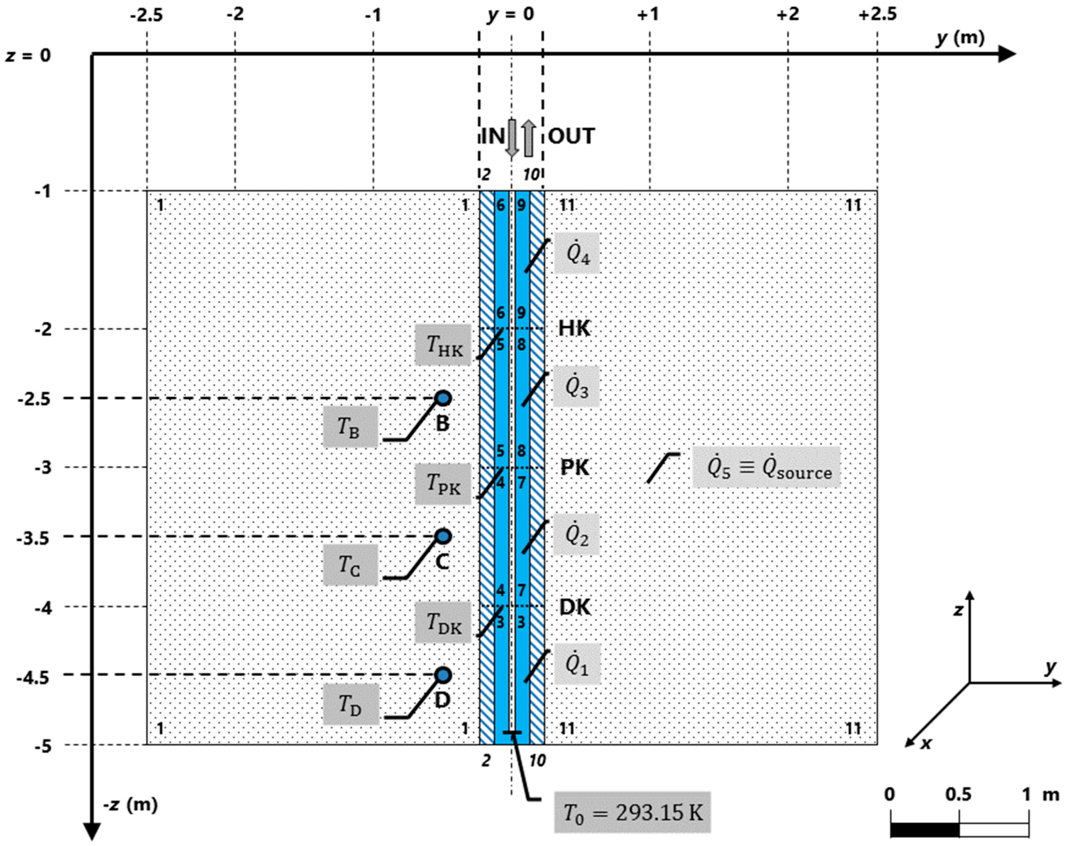
Figure 1.
2D conceptual model: location of the domains and their notification, heat sources, initial value of thermodynamic temperature, and chosen coordinate system (yz-plane).
Figure 1.
2D conceptual model: location of the domains and their notification, heat sources, initial value of thermodynamic temperature, and chosen coordinate system (yz-plane).
Figure 2.
Concept of the solution of the stationary job—block scheme and data flow diagram of the preprocessing (treating input data from chambers and evaluation points), processing (iteration data exchange between the COMSOL model and Matlab custom code via the use of the LiveLink for MATLAB), and postprocessing (treating output data depending on the optimization type) parts.
Figure 3.
The case study I: Q-T diagram for evaluation points B (depth: −2.5 m), C (depth: −3.5 m), and D (depth: −4.5 m) with determined approximated parameters of the line and corrected values of the positive heat sources , , and (Watts) for particular thermodynamic temperatures , , and (Kelvins); stationary job, 2D model.
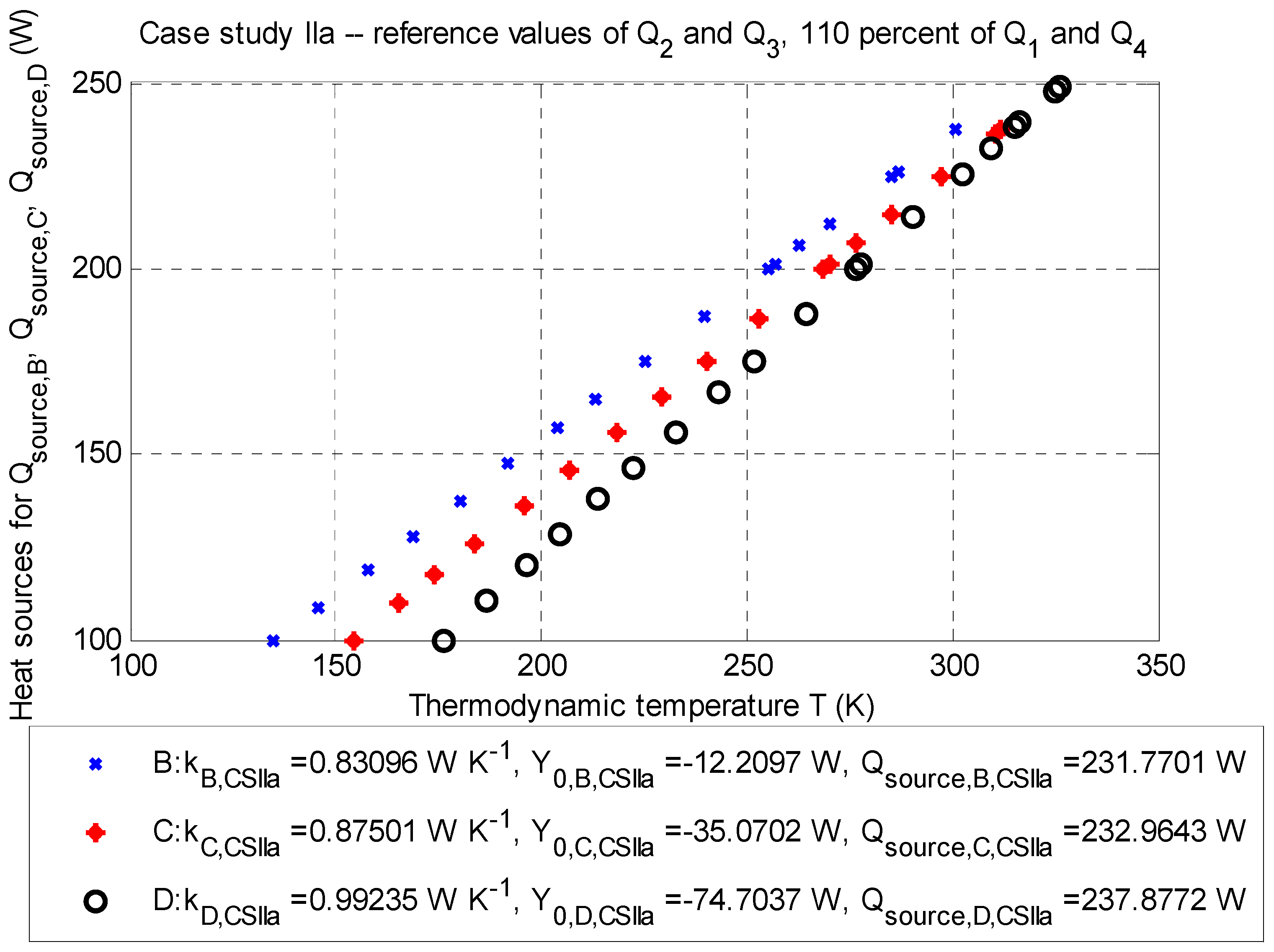
Figure 4.
Case study IIa: Q-T diagram for evaluation points B (depth: −2.5 m), C (depth: −3.5 m), and D (depth: −4.5 m) with determined approximated parameters of the line and corrected values of the positive heat sources , and (Watts) for particular thermodynamic temperatures , and (K); stationary job, 2D model.
Figure 5.
Case study IIb: Q-T diagram for evaluation points B (depth: −2.5 m), C (depth: −3.5 m), and D (depth: −4.5 m) with the determined approximated parameters of the line and corrected values of the positive heat sources , , and (Watts) for particular thermodynamic temperatures , , and (K); stationary job, 2D model.
Figure 6.
Case study IIIa—Q-T diagram for evaluation points B (depth: −2.5 m), C (depth: −3.5 m), and D (depth: −4.5 m) with the determined approximated parameters of the line and corrected values of the positive heat sources , , and (Watts) for particular thermodynamic temperatures , and (Kelvins); stationary job, 2D model.
Figure 7.
Case study IIIb: Q-T diagram for evaluation points B (depth: −2.5 m), C (depth: −3.5 m), and D (depth: −4.5 m) with the determined approximated parameters of the line and corrected values of the positive heat sources , , and (Watts) for particular thermodynamic temperatures , , and (Kelvins); stationary job, 2D model.
Figure 8.
All case studies: Comparison of the results for point optimization (and correction to known values of the thermodynamic temperature at a given evaluation point) to measured data (reference value ) via the use of the mean-square error (Kelvins); stationary job, 2D model.
Figure 8.
All case studies: Comparison of the results for point optimization (and correction to known values of the thermodynamic temperature at a given evaluation point) to measured data (reference value ) via the use of the mean-square error (Kelvins); stationary job, 2D model.
Figure 9.
All case studies: Comparison of the results for the thermal profile to measured data (reference value ) via the use of the mean-square error (Kelvins); stationary job, 2D model.
Figure 9.
All case studies: Comparison of the results for the thermal profile to measured data (reference value ) via the use of the mean-square error (Kelvins); stationary job, 2D model.
Table 1.
The Hedwig mining dump–basic technical parameters (see also [
10]).
Table 1.
The Hedwig mining dump–basic technical parameters (see also [
10]).
| Parameter | Value | Unit |
|---|
| dump’s soil volume | 4.2 × 10⁶ | m3 |
| dump’s area | 32.0 × 10⁴ | m2 |
| the average thickness of the loose body | 15 | m |
| maximal thickness of the loose body | 40 (locally) | m |
| Dump’s operation period | 1900–1998 | ------ |
| the technology of transporting an excavated material | using mine trucks | ------ |
| the technology of storing excavated material | successive dumping into a valley system | ------ |
Table 2.
Mathematical model—values of the chosen physical parameters in the target object Heat Source 5 based on the percentage content of particular rocks.
Table 2.
Mathematical model—values of the chosen physical parameters in the target object Heat Source 5 based on the percentage content of particular rocks.
| Parameter | Value | Unit |
|---|
| Sandstone | Siltstone | Claystone | Result |
|---|
| ------ | | ------ | | ------ |
|---|
| 0.18 | 2.000 | 0.50 | 2.300 | 0.32 | 2.200 | 2.214 | W∙m−1∙K−1 |
| 2500 | 2600 | 2600 | 2582 | kg∙m−3 |
| 2.000 × 10⁶ | 2.300 × 10⁶ | 2.300 × 10⁶ | 2.246 × 10⁶ | J∙m−3∙K−1 |
| 800.000 | 884.615 | 884.615 | 869.868 | J∙kg−1∙K−1 |
| 1.000 × 10⁻⁶ | 1.000 × 10⁻⁶ | 0.957 × 10⁻⁶ | 0.986 × 10⁻⁶ | m2∙s−1 |
Table 3.
Mathematical model—globally defined parameters of the model in the form of heat sources and their implementation in COMSOL (i.e., the heat sources, domains, and target objects).
Table 3.
Mathematical model—globally defined parameters of the model in the form of heat sources and their implementation in COMSOL (i.e., the heat sources, domains, and target objects).
| Heat Sources | Domains | Target Object |
|---|
| Parameter | Unit | ID | Volume | Unit |
|---|
| W | 3 | 50.9181 × 10⁻³ | m3 | Heat Source 1 |
| W | 4 and 7 | 50.7218 × 10⁻³ | m3 | Heat Source 2 |
| W | 5 and 8 | 50.7218 × 10⁻³ | m3 | Heat Source 3 |
| W | 6 and 9 | 50.7218 × 10⁻³ | m3 | Heat Source 4 |
| W | 1 and 11 | 86.2254 | m3 | Heat Source 5 |
Table 4.
The case study I: Reference values of the negative heat sources to , and estimations of the positive heat source for evaluation points B, C, and D.
Table 4.
The case study I: Reference values of the negative heat sources to , and estimations of the positive heat source for evaluation points B, C, and D.
| Evaluation Points | Heat Sources |
|---|
| | | | |
|---|
| (m) | (W) | (W) | (W) | (W) | (W) |
| B: [0.5; −2.5] | −5.2377 | −12.0464 | −52.3756 | −133.0341 | +213.6783 |
| C: [0.5; −3.5] | +213.6802 |
| D: [0.5; −4.5] | +224.0250 |
| ----- | | ----- |
Table 5.
The case study I: Estimation of the positive heat source , and consequent corrections to thermodynamic temperatures , and and for evaluation points B, C, and D (for points and a thermal profile).
Table 5.
The case study I: Estimation of the positive heat source , and consequent corrections to thermodynamic temperatures , and and for evaluation points B, C, and D (for points and a thermal profile).
| Evaluation Points | Optimization | Correction |
|---|
| | | | |
|---|
| (m) | (W) | (%) | (W) | (%) | (K) |
| B: [0.5; −2.5] | +213.6783 | −1.5392 | +217.0187 | 0 | 293.6104 |
| C: [0.5; −3.5] | +213.6802 | −2.3879 | +218.9076 | 0 | 306.3205 |
| D: [0.5; −4.5] | +224.0250 | −0.0296 | +224.0914 | 0 | 314.9920 |
| B, C, D | +215.5451 | ----- | ----- | ----- | Temperature profile |
Table 6.
Case study IIa: 110% of the reference value of the negative heat sources and , and the nominal values of the heat sources and for evaluation points B, C, and D.
Table 6.
Case study IIa: 110% of the reference value of the negative heat sources and , and the nominal values of the heat sources and for evaluation points B, C, and D.
| Evaluation Points | Heat Sources |
|---|
| | | | |
|---|
| (m) | (W) | (W) | (W) | (W) | (W) |
| B: [0.5; −2.5] | −5.7615 | −12.0464 | −52.3756 | −146.3375 | +226.0771 |
| C: [0.5; −3.5] | +236.5147 |
| D: [0.5; −4.5] | +238.2865 |
| ----- | | ----- |
Table 7.
Case study IIa: Estimations of the positive heat source and consequent corrections to thermodynamic temperatures , , and for evaluation points B, C, and D (for points and a thermal profile).
Table 7.
Case study IIa: Estimations of the positive heat source and consequent corrections to thermodynamic temperatures , , and for evaluation points B, C, and D (for points and a thermal profile).
| Evaluation Points | Optimization | Correction |
|---|
| | | | |
|---|
| (m) | (W) | (%) | (W) | (%) | (K) |
| B: [0.5; −2.5] | +226.0771 | −2.4563 | +231.7701 | +6.7973 | 293.6104 |
| C: [0.5; −3.5] | +236.5147 | +1.5240 | +232.9643 | +6.4213 | 306.3205 |
| D: [0.5; −4.5] | +238.2865 | +0.1721 | +237.8772 | +6.1519 | 314.9920 |
| B, C, D | +228.2198 | ----- | ----- | ----- | Temperature profile |
Table 8.
Case study IIb: 90% of reference values of the negative heat sources and and the nominal values of the heat sources a for evaluation points B, C, and D.
Table 8.
Case study IIb: 90% of reference values of the negative heat sources and and the nominal values of the heat sources a for evaluation points B, C, and D.
| Evaluation Points | Heat Sources |
|---|
| | | | |
|---|
| (m) | (W) | (W) | (W) | (W) | (W) |
| B: [0.5; −2.5] | −4.7139 | −12.0464 | −52.3756 | −119.7307 | +201.1988 |
| C: [0.5; −3.5] | +201.1384 |
| D: [0.5; −4.5] | +211.3246 |
| ----- | | ----- |
Table 9.
Case study IIb: Estimation of the positive heat source and consequent corrections to thermodynamic temperatures , , and for evaluation points B, C, and D (for points and a thermal profile).
Table 9.
Case study IIb: Estimation of the positive heat source and consequent corrections to thermodynamic temperatures , , and for evaluation points B, C, and D (for points and a thermal profile).
| Evaluation Points | Optimization | Correction |
|---|
| | | | |
|---|
| (m) | (W) | (%) | (W) | (%) | (K) |
| B: [0.5; −2.5] | +201.1988 | −0.5283 | +202.2673 | −6.7973 | 293.6104 |
| C: [0.5; −3.5] | +201.1384 | −1.8122 | +204.8508 | −6.4213 | 306.3205 |
| D: [0.5; −4.5] | +211.3246 | +0.4846 | +210.3055 | −6.1519 | 314.9920 |
| B, C, D | +200.9861 | ----- | ----- | ----- | Temperature profile |
Table 10.
Case study IIIa: 110% of the reference values of the negative heat sources and and the nominal values of the heat sources and for evaluation points B, C, and D.
Table 10.
Case study IIIa: 110% of the reference values of the negative heat sources and and the nominal values of the heat sources and for evaluation points B, C, and D.
| Evaluation Points | Heat Sources |
|---|
| | | | |
|---|
| (m) | (W) | (W) | (W) | (W) | (W) |
| B: [0.5; −2.5] | −5.2377 | −13.2510 | −57.6135 | −133.0341 | +223.3922 |
| C: [0.5; −3.5] | +225.2415 |
| D: [0.5; −4.5] | +226.6173 |
| ----- | | ----- |
Table 11.
Case study IIIa: Estimation of the positive heat source and consequent corrections to thermodynamic temperatures , , and for evaluation points B, C, and D (for points and a thermal profile).
Table 11.
Case study IIIa: Estimation of the positive heat source and consequent corrections to thermodynamic temperatures , , and for evaluation points B, C, and D (for points and a thermal profile).
| Evaluation Points | Optimization | Correction |
|---|
| | | | |
|---|
| (m) | (W) | (%) | (W) | (%) | (K) |
| B: [0.5; −2.5] | +223.3922 | −0.2407 | +223.9313 | +3.1852 | 293.6104 |
| C: [0.5; −3.5] | +225.2415 | −0.1543 | +225.5895 | +3.0524 | 306.3205 |
| D: [0.5; −4.5] | +226.6173 | −1.7047 | +230.5475 | +2.8810 | 314.9920 |
| B, C, D | +223.7029 | ----- | ----- | ----- | Temperature profile |
Table 12.
Case study IIIb: 90% of the reference values of the negative heat sources and and the nominal values of the heat sources and for evaluation points B, C, and D.
Table 12.
Case study IIIb: 90% of the reference values of the negative heat sources and and the nominal values of the heat sources and for evaluation points B, C, and D.
| Evaluation Points | Heat Sources |
|---|
| | | | |
|---|
| (m) | (W) | (W) | (W) | (W) | (W) |
| B: [0.5; −2.5] | −5.2377 | −10.8418 | −47.1380 | −133.0341 | +211.3872 |
| C: [0.5; −3.5] | +212.6770 |
| D: [0.5; −4.5] | +213.5146 |
| ----- | | ----- |
Table 13.
Case study IIIb: Estimation of the positive heat source and consequent corrections to thermodynamic temperatures , , and for evaluation points B, C, and D (for points and a thermal profile).
Table 13.
Case study IIIb: Estimation of the positive heat source and consequent corrections to thermodynamic temperatures , , and for evaluation points B, C, and D (for points and a thermal profile).
| Evaluation Points | Optimization | Correction |
|---|
| | | | |
|---|
| (m) | (W) | (%) | (W) | (%) | (K) |
| B: [0.5; −2.5] | +211.3872 | +0.6095 | +210.1065 | −3.1851 | 293.6104 |
| C: [0.5; −3.5] | +212.6770 | +0.2125 | +212.2260 | −3.0522 | 306.3205 |
| D: [0.5; −4.5] | +213.5146 | −1.8935 | +217.6356 | −2.8809 | 314.9920 |
| B, C, D | +211.4523 | ----- | ----- | ----- | Temperature profile |


