ANN-Based Airflow Control for an Oscillating Water Column Using Surface Elevation Measurements

Abstract

Oscillating water column (OWC) plants face power generation limitations due to the stalling phenomenon. This behavior can be avoided by an airflow control strategy that can anticipate the incoming peak waves and reduce its airflow velocity within the turbine duct. In this sense, this work aims to use the power of artificial neural networks (ANN) to recognize the different incoming waves in order to distinguish the strong waves that provoke the stalling behavior and generate a suitable airflow speed reference for the airflow control scheme. The ANN is, therefore, trained using real surface elevation measurements of the waves. The ANN-based airflow control will control an air valve in the capture chamber to adjust the airflow speed as required. A comparative study has been carried out to compare the ANN-based airflow control to the uncontrolled OWC system in different sea conditions. Also, another study has been carried out using real measured wave input data and generated power of the NEREIDA wave power plant. Results show the effectiveness of the proposed ANN airflow control against the uncontrolled case ensuring power generation improvement.

1. Introduction

Ocean energy is a more advantageous renewable resource compared to solar and wind. It is more reliable since it is consistent throughout the day and night and more predictable, which can be foreseen several days in advance, and has significantly denser energy. Oceans represent two-thirds of the earth’s surface and store the energy emitted by the sun, making up the largest source of renewable energy. The energy within may be harnessed in various forms, such as ocean waves, ocean currents, tidal range, tidal currents, ocean thermal energy, and salinity gradients [1,2]. However, despite all of these points, these industries are still underdeveloped [3].

Many ocean energy technologies have emerged to exploit this resource, especially for tidal and wave conversion systems. Both technologies are predicted to contribute the most to the European energy platform in the short to medium term (2025–2030) [4,5]. However, the majority of ocean energy-related industries are still in the early stage of development, ranging from theory, design, up to the demonstration phases [6]. In wave energy conversion, converters of various types can be found across Europe, including oscillating water columns like Limpet in Scotland and NEREIDA in Spain [7], point absorber buoys like PowerBuoy in the UK [8], surface attenuators like the Pelamis in Portugal [9], overtopping devices like the Wave Dragon in Denmark [10], converters for tidal energy conversion, including horizontal axis turbines like SeaGen in Ireland [11], vertical axis turbines like Kobold in Italy [12], and variable foil turbines like the Stingray in the UK [13].

Energy hoarded in waves is the form of ocean energy with the highest deployment potential in European waters. It is known that the waves have a global energy potential 30 times higher than that of tides [5]. Moreover, the latest progress of developed wave energy converters (WEC) and projects offered favorable outcomes, which advanced the wave industry to competitive ranks. These factors attracted the attention of investors and policymakers to wave energy; this has been noticed in some countries that started to assess the abundant resource for possible projects, including Hawaii, Italy, India, Peru, and many others [14,15,16,17]. For countries with advanced projects, efforts were invested in the deployment and integration of full-scale converters, which led some technologies to break into commercial implementations [7,18,19]. By slowly earning more and more confidence from investors and efforts to help research and development of ocean energy, industries started to increase. In fact, the EU-funded related research themes where 68% of the funds were invested in technology development divided into 45% for wave technology development and 23% for tidal technology development [20]. Nowadays, new developments are aiming to maintain this confidence by focusing on reliability, robustness, and reduction of costs and risks [21].

One of the most employed WECs is the oscillating water column (OWC) for its simplicity and feasibility. However, OWCs with Wells turbine-based PTO systems suffer from the stalling effect, which hinders the turbine’s efficiency, leading to a decrease in the energy extraction and limitation of the generated power [22,23]. This paper presents the modeling and control of an OWC system. The proposed control strategy aims to help the PTO avoid the power limitation from the stalling effect. In this context, a novel ANN-based airflow control has been designed and implemented with the objective of controlling an air valve inside the capture chamber of the OWC. This will allow the regulation of the airflow velocity below the critical point that provokes the stalling behavior by considering the wave input characteristics. The ANN has been trained using real wave data measured at the coast of Mutriku using an acoustic doppler current profiler (ADCP), and its capabilities were adopted to recognize the incoming peak waves causing the stalling behavior and provide the adequate reference value of the desired airflow speed for the airflow control scheme.

An airflow control strategy has been proposed to OWC converters to control the airflow rate through the turbine, which should be prevented from exceeding the threshold value beyond which severe internal aerodynamic blade stalling reduces the power output. This is achieved by using a throttle valve (in series) or a by-pass valve (in parallel), as suggested by Falcão et al. in [24]. This strategy has been further implemented using various control approaches, such as the PID controllers used by Amundarain et al. [25], and Mishra et al. improved the control scheme by using fractional order PID (FOPID) in [26], which offered to the controller more flexibility in regular and irregular waves. Later intelligent tuning techniques were introduced by M’zoughi et al. using advanced metaheuristic optimization algorithms and fuzzy gain scheduling (FGS) in [27].

Artificial neural networks are able to efficiently approximate and interpolate multivariate data that would require massive databases [28]. The ANN approach is acknowledged for nonlinear statistical fitting applications [29,30]. Automatic control applications and control design applications have adopted ANN in many nonlinearity problems [31,32,33]. The nonlinearity aspect and complexity of the oscillating water column system makes the ANN a very promising solution to deal with the stalling behavior problem.

Recently, the world has generated electric power from wind turbines, but the airflow control strategy for wind turbines has uncertainty. However, with the developments in meteorological temperature and humidity predictions from Fourier-statistical analysis of hourly data, which guarantees its operation [34,35,36], the temperature readings for all the 365 days and the 24 h may provide a strong stochastical connection to the classic strategy. Likewise, the neural network models were able to perform cold wind control [37,38,39]. Consequently, knowledge through measurements of climatic variables is the amount of airflow received per unit area, which explains the weather records used to estimate airflow on wind turbines available at a certain point on the surface of the earth. Therefore, the best option for a perpetual energy solution is obtaining electricity from mechanical energy generated by the movement of sea waves [40,41,42].

The rest of this paper is organized as follows; Section 2 presents the model statement by mathematically describing the different parts of the OWC plant. The problem statement is presented in Section 3 by introducing the stalling behavior and its effect on the produced torque. Section 4 explains the proposed ANN-based airflow control and the designed ANN reference generator. Section 5 sets a demonstrative study case to study the effectiveness of the proposed ANN-airflow control in different wave conditions. Finally, Section 6 finishes the article with some concluding remarks.

2. Model Statement

This section presents the modeling of the parts of the wave energy converter under study, which is the oscillating water column shown in Figure 1. This includes the mathematical models of the waves, capture chamber, Wells turbine, and the generator.

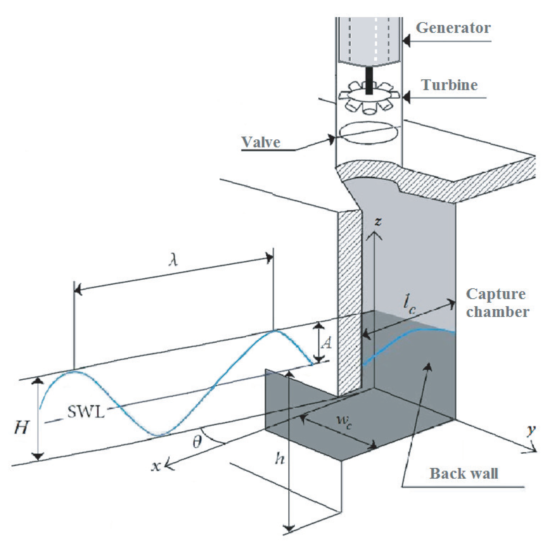
2.1. Wave Surface Dynamics

In this article, monochromatic unidirectional waves are considered as the input to the numerical model of the plant. To describe its surface dynamics, various wave theories may be used, such as Cnoidal wave theory, second or higher-order Stokes theory, and Airy linear theory [43,44].

The simplest description of ocean waves and the most widely used is the Airy wave theory. It expresses the waves as ideal sinusoidal waves by neglecting turbulence, friction losses, and other energy losses [44].

The outline of an ocean wave is illustrated in Figure 1, where $SWL$ is the still water level, h is the sea depth from the seabed to $SWL$. H is wave height from the wave trough to the wave crest. A is the wave amplitude from $SWL$ to the wave crest, and $\lambda$ is the wavelength, which is the distance between successive crests [44,45].

Hence, the surface elevation of an ocean wave may be written as [46,47]:

$$z(x,t)=Asin\left(\omega t-kx\theta \right)=H/2sin\left(\omega t-kx\theta \right)$$

(1)

where x is a horizontal coordinate in which the positive direction is the direction of wave propagation, with $x=0$ at the back wall, $\theta$ is the angle between the x-axis and the direction of wave advance, and k is the wave number, which is related to $\omega$ by the dispersion relationship of Equation (2) defined in [46].

$$ktanh\left(kh\right)={\omega }^2/g$$

(2)

where $\omega$ is the wave frequency, and g is the acceleration gravity.

2.2. Capture Chamber Model

The air volume in the chamber of an OWC is given in [48,49,50] as:

$$V\left(t\right)=V_c+\frac{w_{c}H}{k}sin\left(k{l}_c/2\right)sin\left(\omega t\right)$$

(3)

where $V_c$, $w_c$, and $l_c$ are the capture chamber’s volume, inner width, and length, respectively.

From Equation (3), the volume flow rate may be described as [48,49,50]:

$$Q\left(t\right)=w_{c}cHsin\left(\frac{k{l}_c}{2}\right)cos\left(\omega t\right)$$

(4)

with $c=w_c/k$.

By using Equation (4) and taking into consideration the topology of the capture chamber, the axial airflow speed may be defined as [48,49,50]:

$$v_x\left(t\right)=\frac{Q\left(t\right)}{S}=\frac{8Ac{w}_c}{\pi D^2}sin\left(\frac{\pi l_c}{c{T}_w}\right)cos\left(\frac{2\pi }{T_w}t\right)$$

(5)

where D is the duct diameter.

2.3. Wells Turbine Model

The turbine under study, shown in Figure 2, was invented by Dr. Allan Wells in the mid-1970s [47,51] and is a self-rectifying axial-flow turbine, which provides a unidirectional rotational movement regardless of the airflow direction thanks to its special geometry [52,53].

The Wells turbine may be described by the equations given in [23]:

$$\begin{array}{ccc}\hfill dp& =& C_{a}K\left(1/\phantom{1a}a\right)\left[v_x^2+{\left(r{\omega }_r\right)}^2\right]\hfill \end{array}$$

(6)

$$\begin{array}{ccc}\hfill K& =& \rho lbn/2\hfill \end{array}$$

(7)

$$\begin{array}{ccc}\hfill T_t& =& r{C}_{t}K\left[v_x^2+{\left(r{\omega }_r\right)}^2\right]\hfill \end{array}$$

(8)

$$\begin{array}{ccc}\hfill \varphi & =& v_x{\left(r{\omega }_r\right)}^{-1}\hfill \end{array}$$

(9)

$$\begin{array}{ccc}\hfill Q& =& a{v}_x\hfill \end{array}$$

(10)

$$\begin{array}{ccc}\hfill {\eta }_t& =& T_t{\omega }_r{\left(dpQ\right)}^{-1}=C_t{\left(C_a\varphi \right)}^{-1}\hfill \end{array}$$

(11)

where $dp$ is the pressure drop, $C_a$ and $C_t$ are, respectively, the power and torque coefficients, $\varphi$ is the flow coefficient, $T_t$, ${\eta }_t$, K, r are, respectively, the turbine’s torque, performance, constant, and mean radius, l, b, n are, respectively, the blade’s chord length, height, and number, ${\omega }_r$ is the angular velocity, a is the cross-sectional area, and $\rho$ is the air density.

The curves of both the power coefficient $C_a$ and the torque coefficient $C_t$ against the flow coefficient $\varphi$ form the characteristic curves of the studied Wells turbine, which are presented in Figure 3.

2.4. Doubly Fed Induction Generator Model

The DFIG model may be described by the equations given in [54,55,56].

The voltages across the stator and rotor in the $dq$ frame may be written as [54,55,56]:

$$\begin{array}{c}\hfill \left\{\begin{array}{c}{\displaystyle v_{ds}=R_s{i}_{ds}+\frac{d{\psi }_{ds}}{dt}-{\omega }_s{\psi }_{qs}}\\ {\displaystyle v_{qs}=R_s{i}_{qs}+\frac{d{\psi }_{qs}}{dt}+{\omega }_s{\psi }_{ds}}\end{array}\right.\end{array}$$

(12)

$$\begin{array}{c}\hfill \left\{\begin{array}{c}{\displaystyle v_{dr}=R_r{i}_{dr}+\frac{d{\psi }_{dr}}{dt}-{\omega }_r{\psi }_{qr}}\\ {\displaystyle v_{qr}=R_r{i}_{qr}+\frac{d{\psi }_{qr}}{dt}+{\omega }_r{\psi }_{dr}}\end{array}\right.\end{array}$$

(13)

where $R_s$ and $R_r$ are the stator and the rotor resistances, ${\omega }_s$ and ${\omega }_r$ are the stator and the rotor angular velocities, $i_{ds}$ and $i_{qs}$ are the d-q stator currents, $i_{dr}$ and $i_{qr}$ are the d-q rotor currents.

The flux linkage in the stator and the rotor may be written as:

$$\begin{array}{c}\hfill \left\{\begin{array}{c}{\displaystyle {\psi }_{ds}=L_{ss}{i}_{ds}+L_m{i}_{dr}}\\ {\displaystyle {\psi }_{qs}=L_{ss}{i}_{qs}+L_m{i}_{qr}}\end{array}\right.\end{array}$$

(14)

$$\begin{array}{c}\hfill \left\{\begin{array}{c}{\displaystyle {\psi }_{dr}=L_{rr}{i}_{dr}+L_m{i}_{ds}}\\ {\displaystyle {\psi }_{qr}=L_{rr}{i}_{qr}+L_m{i}_{qs}}\end{array}\right.\end{array}$$

(15)

where ${\displaystyle L_{ss}}$ and $L_{rr}$ are the stator and the rotor inductances, and $L_m$ is the magnetizing inductance.

The generated electromagnetic torque may be expressed as:

$${\displaystyle T_e=\frac{3}{2}p\left({\psi }_{ds}{i}_{qs}-{\psi }_{qs}{i}_{ds}\right)}$$

(16)

where p is the pair pole number.

The mechanical interaction between the turbine and the generator can be defined as:

$$\frac{J}{p}\frac{d{\omega }_r}{dt}=T_e-T_t$$

(17)

where J is the inertia of the system.

3. Problem Statement

The OWC understudy consists of a Wells turbine coupled to DFIG, however, as already mentioned, the aerodynamics of the turbine gets affected by the stalling phenomenon when reaching a critical flow rate value. In fact, this behavior occurs when the airflow velocity $v_x$ rises quickly, but the slow dynamics of the DFIG prevent the rotational speed ${\omega }_r$ from changing as quick. The stalling effect can be deduced from Figure 3b, which indicates that when the flow coefficient $\varphi$ surpasses a certain threshold (which is $0.3$ for this turbine), the torque coefficient $C_t$ drops drastically.

The flow coefficient $\varphi$ described by Equation (9) depends on the airflow speed $v_x$. However, as described by Equation (5), $v_x$ depends on the wave amplitude and period. In fact, the higher the wave amplitude and the shorter the period are, the stronger the wave power and the airflow speed are, as explained by Figure 4.

The stalling effect is shown by studying the uncontrolled OWC plant in two sea conditions; the first one is a wave with a 10 s period and a wave amplitude of 0.9 m starting from 0 s to 22.5 s and the second one is a wave with a 10 s period and a wave amplitude of 1.2 m from 22.5 to 50 s. Figure 5 shows that the first sea condition provides a flow coefficient lower than the threshold value 0.3, whereas, with the second sea condition, it exceeds the threshold value.

Accordingly, the obtained torques shown in Figure 6 indicate no stalling for the first sea condition and a drastic decrease at the crest in the second sea condition by the stalling effect. This will decrease the produced torque in terms of the average value.

4. Control Statement

The stalling phenomenon of the Wells turbine may be avoided by continuously adjusting the flow coefficient [48,49]. By referring to Equation (7), the flow coefficient depends on the airflow speed in the turbine duct. Hence, regulating the airflow velocity $v_x$ will help avoid the stalling effect. In this sense, an ANN-based airflow control scheme has been proposed to control the air valve situated inside the capture chamber of the OWC system in order to regulate the airflow speed $v_x$, thus keeping the flow coefficient $\varphi$ under the threshold value. The ANN will be trained to recognize incoming waves from measured data by the acoustic doppler current profiler (ADCP). The scheme of the proposed ANN-airflow control strategy is presented in Figure 7.

4.1. ANN-Based Airflow Control

The capture chambers in NEREIDA are equipped with air valves at the summit connecting to the turbine duct. The valve is mounted in series with the Wells turbine, followed by the DFIG, as illustrated in Figure 7. It separates the air and pressure in the chamber from that of the capture chamber, and its role is to prevent the pressure difference from surpassing its critical limit [50]. However, this device is also useful in controlling the amount of airflow input. The valve is operated through its actuator, which turns the valve plate to the desired angular position and then holds it by an electromagnetic brake. The flow rate will vary depending on the degree of the opening of the valve plate.

This control strategy aims to control the air valve using a proportional integral (PI) controller, as explained by the block diagram of Figure 8. This is achieved by measuring the airflow velocity in the turbine duct $V_X^{\prime }$ and comparing it to the reference velocity $V_{XRef}$. The reference velocity $V_{XRef}$ is provided by the ANN airflow velocity reference generator. The output of the PI controller is the control signal for the valve actuator.

The ANN will be trained to recognize incoming waves from measured data gathered by AZTI-Tecnalia at the breakwater of Mutriku in the northern coast of Spain. Both inputs of the designed ANN are obtained from the acoustic doppler current profiler (ADCP) installed at Mutriku (shown in Figure 9). The considered data are from 12 May 2014, where measurements of the first 20 min were recorded every 2 h. The installed ADCP is of Workhorse 600 kHz from Teledyne RDI with a sampling period of 0.5 s.

ADCPs are hydro-acoustic devices used to measure water current velocities. This technology uses the Doppler effect of sound waves scattered back from particles. It is able to send and receive sound signals thanks to piezoelectric transducers. The time it takes sound waves to travel allows estimating the distance. The frequency shift of the echo is proportional to the water velocity within the acoustic path. Three-dimensional velocity measurements require a minimum of three beams [57,58].

In the last few years, more functionality has been added to ADCPs to include wave and turbulence measurements. The ADCP device specific to wave characteristic measurements is known as the acoustic wave and current (AWAC) profiler, which allows the measurement of surface wave height and its direction [59,60]. The one installed in Mutriku is mounted upwards down at the seafloor. The AWAC device has four transducers that transmit four beams; one transducer in the middle point vertically up, and three transducers symmetrically positioned at 120 degrees from each other and surrounding the center one, and they are angled off the vertical by 25 degrees [61,62].

4.2. ANN Airflow Velocity Reference Generator

The trained ANN has to generate reference airflow velocity that does not provoke the stalling behavior of the Wells turbine, this means that when the wave power is low, the total airflow is admitted by the valve, but when the waves are strong enough to generate high airflow speed, the valve should block the incoming airflow to reduce its speed. In this sense, numerous simulations were carried out to record the acceptable waves and distinguish the strong waves that provoke the stalling effect. Hence, input–output data sets have been assembled to train the network into generating the desired output. The desired airflow reference as a function of the wave amplitude and period is shown in Figure 10.

The ANN developed is a feed-forward network controller that consists of an input layer of two neurons; one for the wave amplitude, and the other one for the wave period, and an output layer with one neuron representing the desired airflow speed reference. Determining the number of hidden layers/neurons in such a complex system is an intricate task; therefore, the trial-and-error rule based on the forward approach procedure has been used [63]. The method begins with an undersized number of hidden layers/neurons and then increases them. At every time, the new network structure is trained and tested. This process is repeated until the train and test results are improved. By statistical analysis, the best structure is selected by choosing the best mean squared error (MSE).

ANNs consist of neurons in the input, output, and hidden layers, which are connected with weighted signals ($w_{ij}$). The neurons consist of a bias $b_j$, a sum function $S_j$ coupled to an activation function ${\phi }_j$. The sum function may be defined as:

$$S_j=\sum _{j=1}^N\left(w_{ji}{y}_i\right)+b_j$$

(18)

where $S_j$ is the sum from the $j^{th}$ neuron from the current layer, $b_j$ is the bias, N is the total number of neurons, $w_{ji}$ is the weight of the signal connecting the $j^{th}$ neuron from the current layer with the $i^{th}$ neuron from the previous layer, and $y_i$ is the input signal from the neuron of the previous layer.

The activation function of neurons in the input layer is clamped by the input vector; however, the activation function of the rest of the neurons in the network can be chosen as:

$$y_j={\phi }_j\left(S_j\right)=\left\{\begin{array}{c}{S}_j\left(Linear\right)\hfill \\ \frac{1}{1+e^{-S_j}}\left(Sigmoid\right)\hfill \\ \frac{e^{S_j}-e^{-S_j}}{e^{S_j}+e^{-S_j}}\left(Hyperbolictangent\right)\hfill \end{array}\right.$$

(19)

To train the ANN, the Levenberg–Marquardt (LM) algorithm has been considered as a learning method [64]. This algorithm is a variant of Newton’s method, which was designed to minimize functions that are sums of squares of nonlinear functions [65]. The algorithm aims to update the network weights in order to minimize the performance index by [66]:

$$∆X={\left[{\nabla }^{2}F\left(X\right)\right]}^{-1}\nabla F\left(X\right)$$

(20)

where $F\left(X\right)$ is the performance index, $\nabla F\left(X\right)$ is the gradient, and ${\nabla }^{2}F\left(X\right)$ the Hessian matrix.

Knowing that the performance index is defined as:

$$F\left(X\right)=\sum _{i=1}^N{E}_i^2\left(X\right)=E^T\left(X\right).E\left(X\right)$$

(21)

where $E\left(X\right)$ is the error between the ANN’s output and the target output.

The gradient of the performance index may be written as:

$$\nabla F\left(X\right)=2J^T\left(X\right).E\left(X\right)$$

(22)

where $J\left(X\right)$ is the Jacobian matrix defined as [67]:

$$J\left(X\right)=\left(\begin{array}{cccc}\frac{\partial E_1\left(X\right)}{\partial X_1}& \frac{\partial E_1\left(X\right)}{\partial X_2}& \dots & \frac{\partial E_1\left(X\right)}{\partial X_n}\\ \frac{\partial E_2\left(X\right)}{\partial X_1}& \frac{\partial E_2\left(X\right)}{\partial X_2}& \dots & \frac{\partial E_2\left(X\right)}{\partial X_n}\\ ⋮& ⋮& \ddots & ⋮\\ \frac{\partial E_N\left(X\right)}{\partial X_1}& \frac{\partial E_N\left(X\right)}{\partial X_2}& \cdots & \frac{\partial E_N\left(X\right)}{\partial X_n}\end{array}\right)$$

(23)

where n is the number of training patterns.

Hence, the Hessian matrix may be expressed as:

$${\nabla }^{2}F\left(X\right)=2J^T\left(X\right).J\left(X\right)+2\sum _{i=1}^N{E}_i\left(X\right).{\nabla }^2{E}_i\left(X\right)$$

(24)

5. Results and Discussion

This section presents the simulations carried out to evaluate the performance of the proposed ANN-based airflow control. To evaluate the performance of the proposed control methodology, the OWC wave power plant has been implemented by a complete wave-to-wire model on Matlab/Simulink, and a comparison between the uncontrolled and controlled cases has been performed.

To implement the OWC model, we considered the parameters obtained from real measurements at the NEREIDA wave power plant. These parameters were provided by the Basque Energy Agency (EVE) and are detailed in

Table 1. Plant parameters from the NEREIDA wave power plant at Mutriku.

Capture Chamber	Wells Turbine	DFIG Generator
$w_c$ = 4.5 m	n = 5	$R_s$ = 0.5968 Ω	$P_{rated}$ = 18.45 kW
$l_c$ = 4.3 m	b = 0.21 m	$R_r$ = 0.6258 Ω	$V{s}_{rated}$ = 400 V
${\rho }_a$ = 1.19 ${\mathrm{kg}/\mathrm{m}}^3$	l = 0.165 m	$L_{ss}$ = 0.0003495 H	$f_{rated}$ = 50 Hz
${\rho }_w$ = 1029 ${\mathrm{kg}/\mathrm{m}}^3$	r = 0.375 m	$L_{rr}$ = 0.324 H	$p=2$
	a = 0.4417 ${\mathrm{m}}^2$	$L_m$ = 0.324 H

.

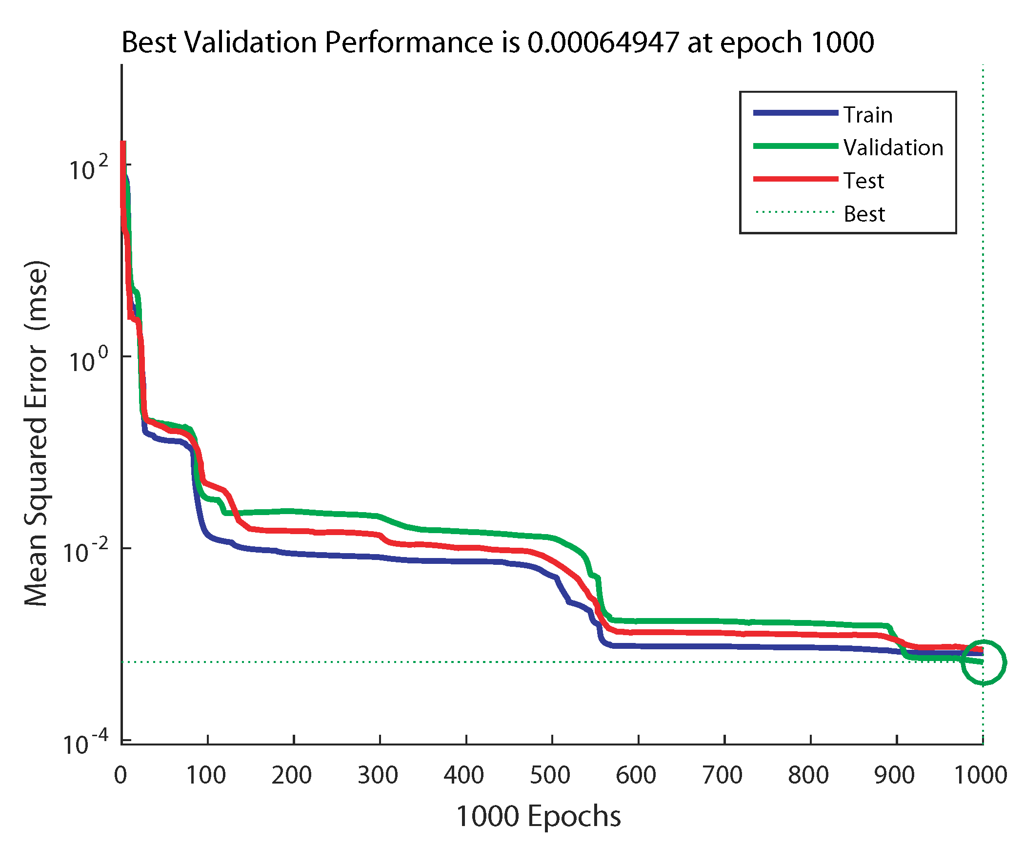
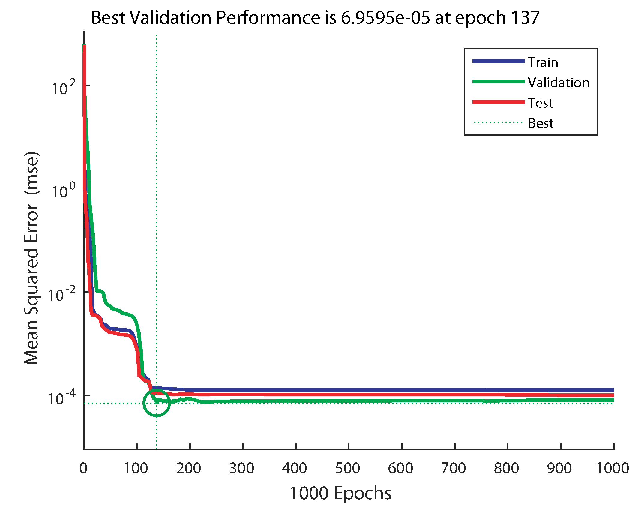
5.1. ANN Training Performance

Using the trial-and-error rule based on the forward approach procedure, several structures with different hidden layers and neurons were tested with our problem in order to obtain the best MSE. The activation function used for the neurons in the hidden layer is the hyperbolic tangent, whereas in the output layer, the linear activation function. During the simulation tests, the comparative study takes into account the number of epochs and the least MSE. The training process was performed on computers with a 3.2 GHz Intel Core i7-8700 Six-Core processor and Integrated Intel UHD Graphics 630.

Table 2. Training performance of different structures using the Levenberg–Marquardt algorithm.

Network Structure	Epochs	MSE	Network Structure	Epochs	MSE
	11	1.1196		237	1.0463 × 10${}^{-3}$
2 × 2 × 1	20	8.0244 × 10${}^{-1}$	2 × 2 × 2 × 1	453	9.8214 × 10${}^{-4}$
	56	7.3278 × 10${}^{-1}$		619	8.1576 × 10${}^{-4}$
	98	3.8778 × 10${}^{-1}$		862	8.6248 × 10${}^{-4}$
	68	1.5626 × 10${}^{-1}$		202	8.5032 × 10${}^{-4}$
2 × 4 × 1	122	9.0921 × 10${}^{-2}$	2 × 4 × 2 × 1	534	7.9368 × 10${}^{-4}$
	566	6.6619 × 10${}^{-2}$		811	8.2294 × 10${}^{-4}$
	698	4.2215 × 10${}^{-2}$		1000	7.6146 × 10${}^{-4}$
	188	4.2318 × 10${}^{-2}$		115	9.0408 × 10${}^{-4}$
2 × 8 × 1	528	5.4049 × 10${}^{-3}$	2 × 2 × 4 × 1	482	7.7924 × 10${}^{-4}$
	706	7.6852 × 10${}^{-3}$	(ANN1)	726	8.1396 × 10${}^{-4}$
	1000	2.3425 × 10${}^{-3}$		1000	6.4947 × 10${}^{-4}$
	307	1.7154 × 10${}^{-3}$		98	8.3164 × 10${}^{-4}$
2 × 16 × 1	423	1.3220 × 10${}^{-3}$	2 × 4 × 4 × 1	137	6.9595 × 10${}^{-5}$
	775	7.3013 × 10${}^{-4}$	(ANN2)	546	8.0274 × 10${}^{-4}$
	1000	8.8384 × 10${}^{-4}$		934	7.0812 × 10${}^{-4}$

shows the results obtained of training different networks with different structures applied to the problem of wave characteristics recognition.

From the results of Table 2, we can deduce that the results obtained using a single hidden layer networks, known as Vanilla neural networks, performs poorly due to the nonlinearity and complexity of the problem. On the other hand, network structures with more than one hidden layer, known as deep neural networks, offer better performance. Therefore, further analysis was carried out on the curves of the training performance of the deep neural network structures, with the best results marked as ANN1 (2 × 2 × 4 × 1) and ANN2 (2 × 4 × 4 × 1) in order to select the adequate structure.

The evolution of the training process of ANN1 (2 × 2 × 4 × 1) is depicted in Figure 11, and the one of ANN2 (2 × 4 × 4 × 1) is depicted in Figure 12. From these figures, it can be noticed that in the case of ANN1, the training process took more epochs to converge to the minimum MSE of 6.4947 × 10${}^{-4}$; however, with ANN2, it converged to a smaller MSE of 6.9595 × 10${}^{-5}$ in fewer epochs at 137.

Finally, the topology of ANN2 has been selected as the ANN airflow velocity reference generator to be implemented in the proposed airflow control scheme to provide the desired airflow speed.

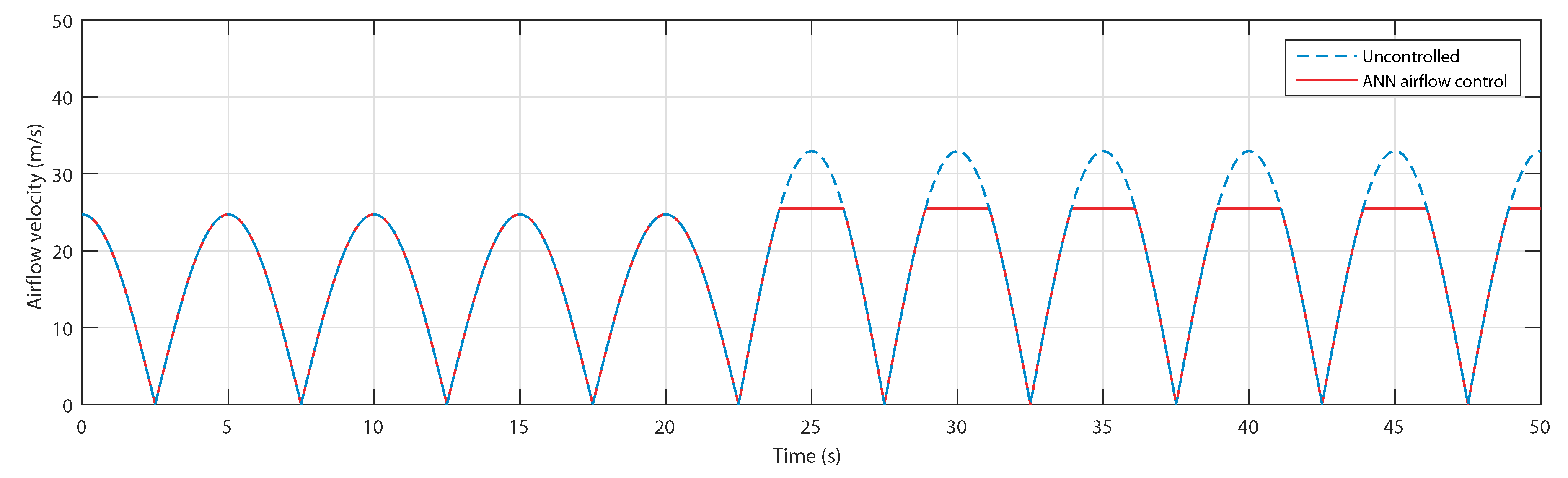
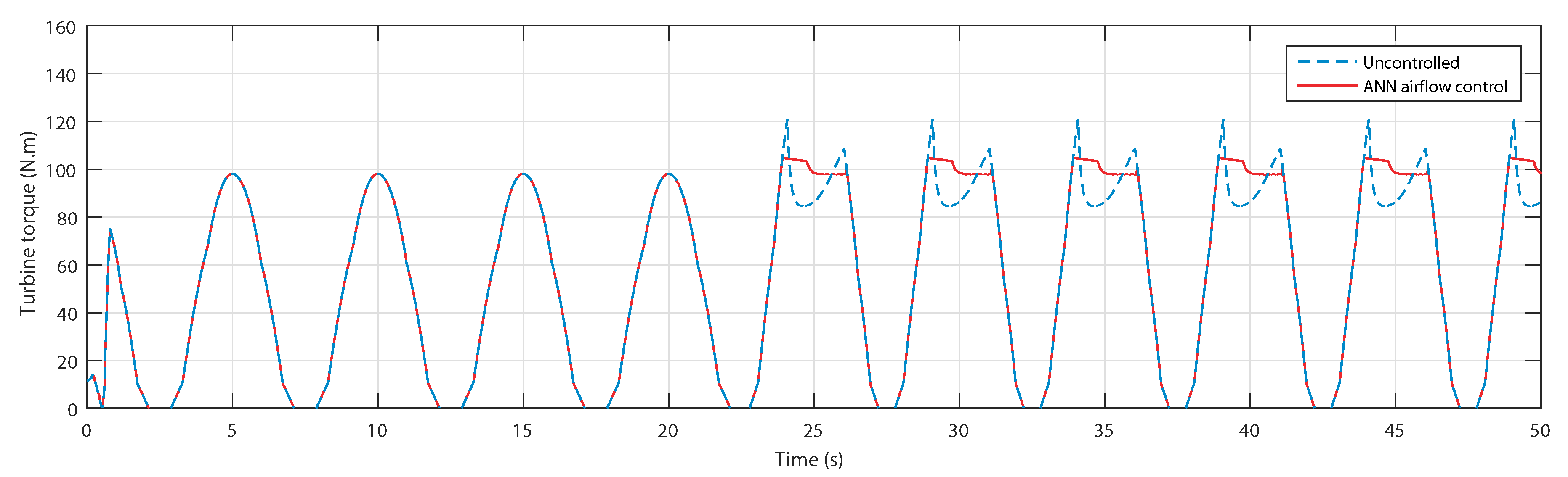
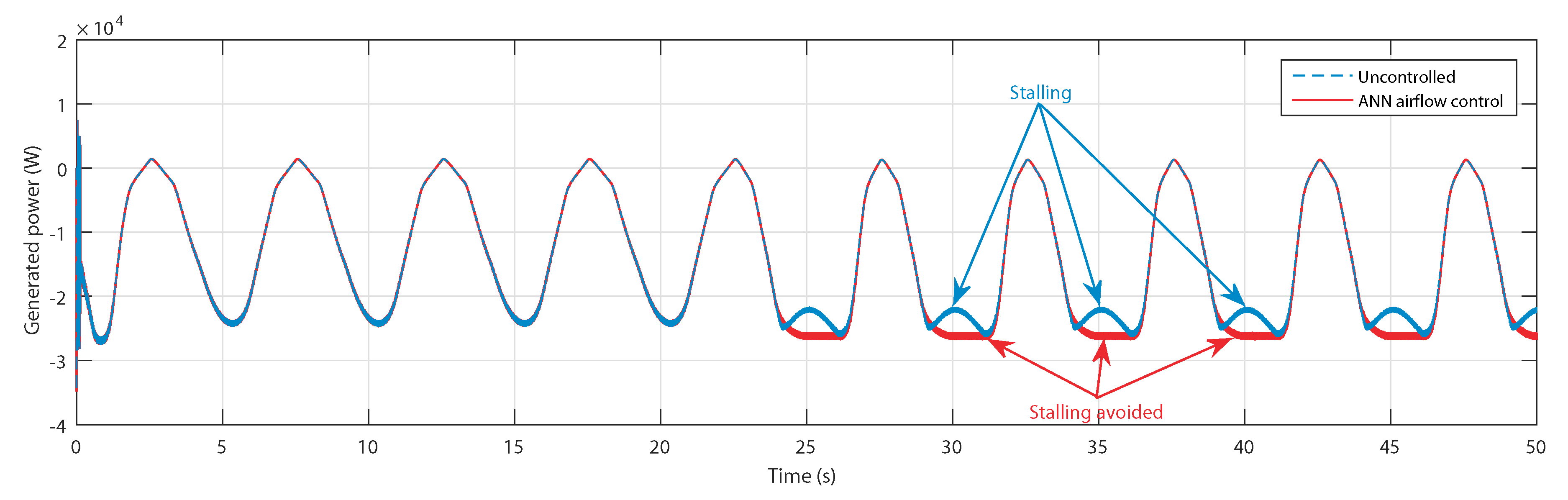
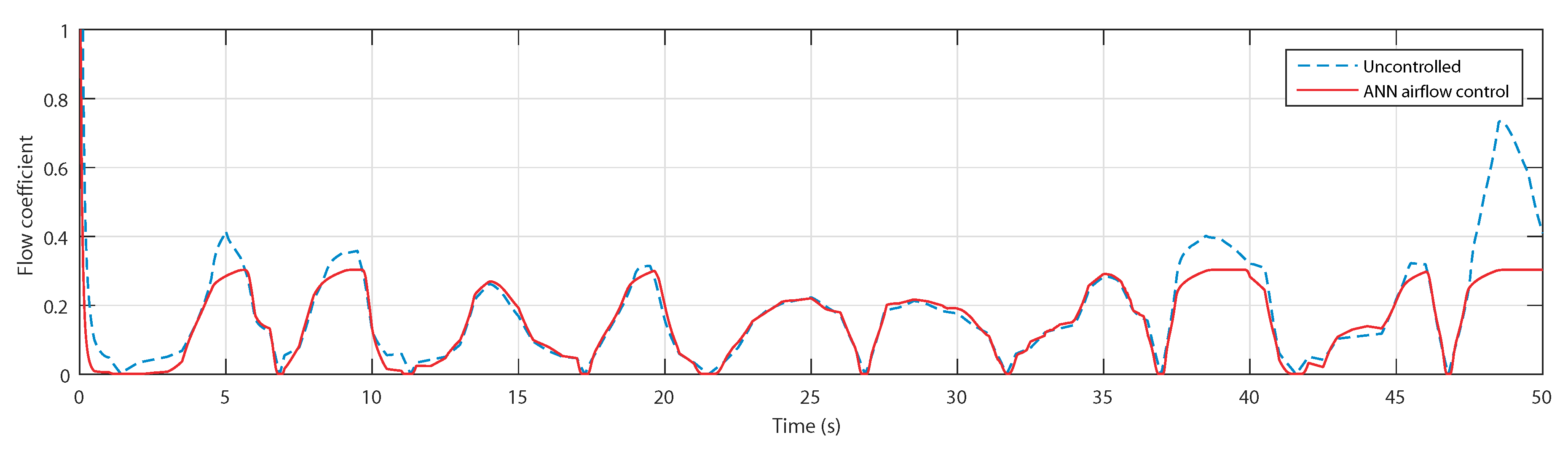
5.2. Control Assessment with Regular Waves

To evaluate the power generation enhancement of the proposed ANN-based airflow control scheme, a study case considering two representative sea states from the site of Mutriku are selected from the wave spectrum of the location illustrated in Figure 13.

The waves are characterized by a water depth $h=$ 5 m and a wave period $T_w=10$ s. The first wave amplitude is $A=0.9$ m from 0 s to 22.5 s, and the second wave amplitude is $A=1.2$ m from 22.5 s to 50 s, as shown in Figure 14.

Figure 15 shows the airflow speed for both waves in the uncontrolled and controlled cases. The curves show that for the first sea condition, the airflow velocity is in the acceptable range, whereas for the second wave, the neural network recognized the wave as one that will provoke a stalling behavior in the OWC; therefore, the control has been activated and the speed has been reduced by the air valve.

The flow coefficients are presented in Figure 16 and show that, indeed, the flow coefficient of the first wave did not exceed the threshold value of $0.3$ in the uncontrolled case, which required no action in the controlled case. However, in the case of the second wave, the flow coefficient did exceed the threshold value; hence, the control managed to successfully adjust it.

The resulting produced torques are shown in Figure 17, where it is clearly observed that with the second wave, the torque in the uncontrolled case has a drastic decrease at every crest, which reduces the torque in terms of average value. However, using the ANN-airflow control, the torque has been maintained at the maximum value, thus maintaining a higher average value.

Eventually, the generated power avoided the power drop at the peak of the second wave, as shown in Figure 18. Therefore, the generated power is higher in terms of the average value with the use of the ANN-based airflow control.

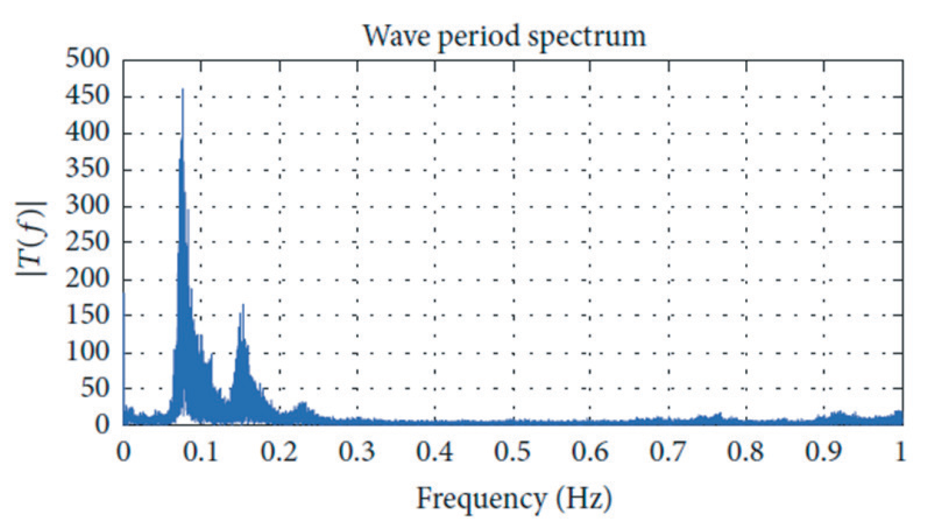
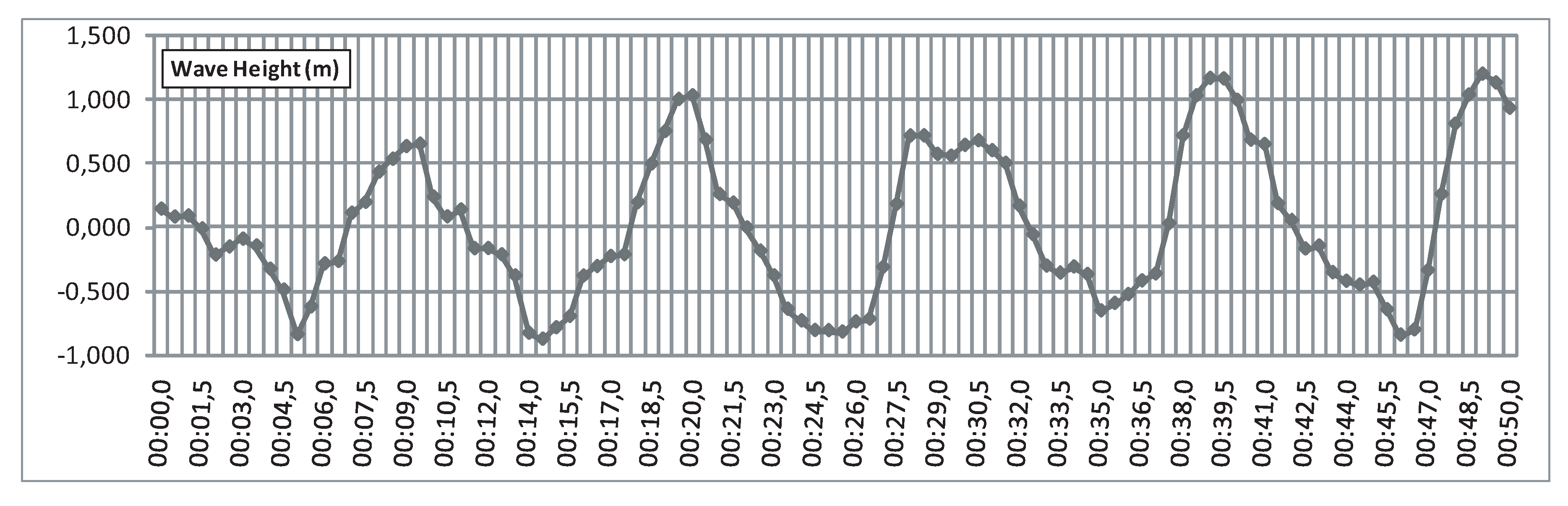
5.3. Control Assessment with Real Measured Wave Data

In this comparative study, we considered real surface elevation measurements of waves in Mutriku obtained by the Acoustic Doppler Current Profiler on 12 May 2014, at 00:00:00, as shown in Figure 19. This measured input will help test the proposed control with other wave amplitudes and periods.

The curves of the airflow speed in Figure 20 showed fast airflow at the peak of the waves, namely at 5, 8, 38, and 48 s. Effectively, the ANN controller activated the airflow control, and the speed has been reduced by the air valve.

Confirming with the curves of the airflow speed, the flow coefficients, shown in Figure 21, have indeed exceeded the threshold value at the indicated instances when uncontrolled. The controlled OWC, however, shows a regulation of the coefficient at the threshold value 0.3.

The torques shown in Figure 22 prove that the uncontrolled torque did indeed suffer from the stall effect at the same instants, but thanks to the airflow control, they were successfully avoided.

Same as the torques, the generated powers have successfully avoided the stalling effect, as indicated in Figure 23.

For a final comparison, Figure 24 shows the output power of the OWC measured in the Mutriku facility at the same time and on the same day (12 May 2014, at 00:00:00). These data were provided by the Basque Energy Agency (EVE).

By taking into consideration the quality of the data series due to the large sampling period, one can see the same waveform in both the numerical power of Figure 23 and Figure 24. However, at the instants 5, 8, 18, 38, and 48 s, the controlled power is superior to the measured power.

6. Conclusions

In this article, the modeling and implementation of an OWC system using a Wells turbine coupled to a DFIG has been presented. The paper also proposes a novel ANN-based airflow control for the OWC to deal with the stalling behavior of the Wells turbine, which proves to limit the generated power.

The proposed ANN-airflow control uses a trained artificial neural network to recognize waves with high airflow speed that may cause a stalling effect in the system. The data used to train the ANN were gathered by an Acoustic Doppler Current Profiler. The ANN is then able to generate an adequate airflow speed reference. The reference is used in the airflow control scheme. To design the suitable network structure for the problem, numerous simulations were performed using the trial-and-error rule based on the forward approach procedure. The best topology has been selected by considering the best performance index MSE, the number of epochs, and the least complicated structure.

The results of the training process showed that the best MSE is obtained with deep neural networks. The considered ANN topology was able to converge in an acceptable number of epochs. Using the trained network in the airflow scheme, the airflow strategy has been able to detect strong waves and avoid the stalling behavior. The results prove the effectiveness of the control with different sea states. Also, a comparative study using real surface elevation measurements of waves in Mutriku showed good avoidance of the stalling phenomenon even compared to the measured power output of the NEREIDA plant in Mutriku.

References

1. Huckerby, J.; Jeffrey, H.; Jay, B.; Executive, O. An International Vision for Ocean Energy; Ocean Energy Systems: Lisbon, Portugal, 2011. [Google Scholar]
2. Brito, A.; Villate, J.L. Annual Report 2014: Implementing Agreement on Ocean Energy Systems; Ocean Energy Systems: Lisbon, Portugal, 2015. [Google Scholar]
3. Lehmann, M.; Karimpour, F.; Goudey, C.A.; Jacobson, P.T.; Alam, M.R. Ocean wave energy in the United States: Current status and future perspectives. Renew. Sustain. Energy Rev. 2017, 74, 1300–1313. [Google Scholar] [CrossRef]
4. Alamir, M.; Fiacchini, M.; Chabane, S.B.; Bacha, S.; Kovaltchouk, T. Active power control under Grid Code constraints for a tidal farm. In Proceedings of the 2016 Eleventh International Conference on Ecological Vehicles and Renewable Energies (EVER), New York, NY, USA, 6–8 April 2016; pp. 1–7. [Google Scholar]
5. Magagna, D.; Uihlein, A. 2014 JRC Ocean Energy Status Report; European Commission: Luxembourg, 2015. [Google Scholar]
6. Rusu, L.; Onea, F. Assessment of the performances of various wave energy converters along the European continental coasts. Energy 2015, 82, 889–904. [Google Scholar] [CrossRef]
7. Heath, T.V. A review of oscillating water columns. Philos. Trans. R. Soc. A Math. Phys. Eng. Sci. 2012, 370, 235–245. [Google Scholar] [CrossRef] [PubMed] [Green Version]
8. Lagoun, M.S.; Benalia, A.; Benbouzid, M.H. Ocean wave converters: State of the art and current status. In Proceedings of the 2010 IEEE International Energy Conference, Manama, Bahrain, 18–22 December 2010; pp. 636–641. [Google Scholar]
9. Yemm, R.; Pizer, D.; Retzler, C.; Henderson, R. Pelamis: Experience from concept to connection. Philos. Trans. R. Soc. A Math. Phys. Eng. Sci. 2012, 370, 365–380. [Google Scholar] [CrossRef] [Green Version]
10. Kofoed, J.P.; Frigaard, P.; Friis-Madsen, E.; Sørensen, H.C. Prototype testing of the wave energy converter wave dragon. Renew. Energy 2006, 31, 181–189. [Google Scholar] [CrossRef] [Green Version]
11. Westwood, A. SeaGen installation moves forward. Renew. Energy Focus 2008, 9, 26–27. [Google Scholar] [CrossRef]
12. Calcagno, G.; Salvatore, F.; Greco, L.; Moroso, A.; Eriksson, H. Experimental and numerical investigation of an innovative technology for marine current exploitation: The Kobold turbine. In Proceedings of the Sixteenth International Offshore and Polar Engineering Conference, San Francisco, CA, USA, 28 May–2 June 2006; pp. 323–330. [Google Scholar]
13. Kinsey, T.; Dumas, G.; Lalande, G.; Ruel, J.; Mehut, A.; Viarouge, P.; Lemay, J.; Jean, Y. Prototype testing of a hydrokinetic turbine based on oscillating hydrofoils. Renew. Energy 2011, 36, 1710–1718. [Google Scholar] [CrossRef]
14. Stopa, J.E.; Cheung, K.F.; Chen, Y.L. Assessment of wave energy resources in Hawaii. Renew. Energy 2011, 36, 554–567. [Google Scholar] [CrossRef]
15. Liberti, L.; Carillo, A.; Sannino, G. Wave energy resource assessment in the Mediterranean, the Italian perspective. Renew. Energy 2013, 50, 938–949. [Google Scholar] [CrossRef]
16. Kumar, V.S.; Anoop, T.R. Wave energy resource assessment for the Indian shelf seas. Renew. Energy 2015, 76, 212–219. [Google Scholar] [CrossRef]
17. López, M.; Veigas, M.; Iglesias, G. On the wave energy resource of Peru. Energy Convers. Manag. 2015, 90, 34–40. [Google Scholar] [CrossRef]
18. Drew, B.; Plummer, A.R.; Sahinkaya, M.N. A review of wave energy converter technology. Proc. Inst. Mech. Eng. A J. Power Energy 2009, 223, 887–902. [Google Scholar] [CrossRef] [Green Version]
19. Antonio, F.D.O. Wave energy utilization: A review of the technologies. Renew. Sustain. Energy Rev. 2010, 14, 899–918. [Google Scholar]
20. Corsatea, T.D.; Magagna, D. Overview of European Innovation Activities in Marine Energy Technology; JRC Science and Policy Reports; European Commission: Brussels, Belgium, 2013. [Google Scholar]
21. European Commission. Report on the Blue Growth Strategy Towards More Sustainable Growth and Jobs in the Blue Economy; European Commission: Brussels, Belgium, 2017; pp. 1–62. Available online: Https://ec.europa.eu/maritimeaffairs/policy/blue_growth_en (accessed on 28 February 2020).
22. Raghunathan, S. Performance of the Wells self-rectifying turbine. Aeronaut. J. 1985, 89, 369–379. [Google Scholar]
23. Raghunathan, S. The wells air turbine for wave energy conversion. Prog. Aerospace Sci. 1995, 31, 335–386. [Google Scholar] [CrossRef]
24. Falcão, A.D.O.; Justino, P.A.P. OWC wave energy devices with air flow control. Ocean Eng. 1999, 26, 1275–1295. [Google Scholar] [CrossRef]
25. Amundarain, M.; Alberdi, M.; Garrido, A.J.; Garrido, I. Modeling and simulation of wave energy generation plants: Output power control. IEEE Trans. Ind. Electron. 2010, 58, 105–117. [Google Scholar] [CrossRef] [Green Version]
26. Mishra, S.K.; Purwar, S.; Kishor, N. Air flow control of OWC wave power plants using FOPID controller. In Proceedings of the 2015 IEEE Conference on Control Applications (CCA), Sydney, Australia, 19–22 September 2016; pp. 1516–1521. [Google Scholar]
27. M’zoughi, F.; Garrido, I.; Bouallègue, S.; Ayadi, M.; Garrido, A.J. Intelligent Airflow Controls for a Stalling-Free Operation of an Oscillating Water Column-Based Wave Power Generation Plant. Electronics 2019, 8, 70. [Google Scholar] [CrossRef] [Green Version]
28. Omidvar, O.; Elliott, D.L. Neural Systems for Control; Academic Press: Cambridge, MA, USA, 1997; ISBN 9780080537399. [Google Scholar]
29. Yilmaz, A.S.; Ozer, Z. Pitch angle control in wind turbines above the rated wind speed by multi-layer perceptron and radial basis function neural networks. Expert Syst. Appl. 2009, 36, 9767–9775. [Google Scholar] [CrossRef]
30. Alberdi, M.; Amundarain, M.; Garrido, A.; Garrido, I. Neural control for voltage dips ride-through of oscillating water column-based wave energy converter equipped with doubly-fed induction generator. Renew. Energy 2012, 48, 16–26. [Google Scholar] [CrossRef]
31. Legowski, A.; Niezabitowski, M. An industrial robot singular trajectories planning based on graphs and neural networks. AIP Conf. Proc. 2016, 1738, 480057. [Google Scholar]
32. Bertachi, A.; Biagi, L.; Contreras, I.; Luo, N.; Vehí, J. Prediction of Blood Glucose Levels And Nocturnal Hypoglycemia Using Physiological Models and Artificial Neural Networks. In Proceedings of the KHD@ IJCAI, Stockholm, Schweden, 13–19 July 2018; pp. 85–90. [Google Scholar]
33. Farooq, Z.; Zaman, T.; Khan, M.A.; Muyeen, S.M.; Ibeas, A. Artificial Neural Network Based Adaptive Control of Single Phase Dual Active Bridge With Finite Time Disturbance Compensation. IEEE Access 2019, 7, 112229–112239. [Google Scholar] [CrossRef]
34. Krzyszczak, J.; Baranowski, P.; Zubik, M.; Hoffmann, H. Temporal scale influence on multifractal properties of agro-meteorological time series. Agric. For. Meteorol. 2017, 239, 223–235. [Google Scholar] [CrossRef]
35. Castañeda-Miranda, A.; Icaza-Herrera, M.D.; Castaño, V.M. Meteorological Temperature and Humidity Prediction from Fourier-Statistical Analysis of Hourly Data. Adv. Meteorol. 2019, 2019, 1–13. [Google Scholar] [CrossRef]
36. Yang, Z.C. Hourly ambient air humidity fluctuation evaluation and forecasting based on the least-squares Fourier-model. Measurement 2019, 133, 112–123. [Google Scholar] [CrossRef]
37. Stoyanov, D.B.; Nixon, J.D. Alternative operational strategies for wind turbines in cold climates. Renew. Energy 2020, 145, 2694–2706. [Google Scholar] [CrossRef]
38. Castañeda-Miranda, A.; Castaño, V.M. Smart frost control in greenhouses by neural networks models. Comput. Electron. Agric. 2017, 137, 102–114. [Google Scholar] [CrossRef]
39. Li, C.; Zhou, D.; Wang, H.; Lu, Y.; Li, D. Techno-economic performance study of stand-alone wind/diesel/battery hybrid system with different battery technologies in the cold region of China. Energy 2020, 192, 116702. [Google Scholar] [CrossRef]
40. Konispoliatis, D.N.; Mavrakos, S.A. Natural frequencies of vertical cylindrical oscillating water column devices. Appl. Ocean Res. 2019, 91, 101894. [Google Scholar] [CrossRef]
41. Zheng, S.; Zhu, G.; Simmonds, D.; Greaves, D.; Iglesias, G. Wave power extraction from a tubular structure integrated oscillating water column. Renew. Energy 2020, 150, 342–355. [Google Scholar] [CrossRef]
42. Singh, U.; Abdussamie, N.; Hore, J. Hydrodynamic performance of a floating offshore OWC wave energy converter: An experimental study. Renew. Sustain. Energy Rev. 2020, 117, 109501. [Google Scholar] [CrossRef]
43. Sobey, R.; Goodwin, P.; Thieke, R.; Westberg, R.J., Jr. Application of Stokes, Cnoidal, and Fourier wave theories. J. Waterway Port Coast. Ocean Eng. 1987, 113, 565–587. [Google Scholar] [CrossRef]
44. Le Roux, J.P. An extension of the Airy theory for linear waves into shallow water. Coast. Eng. 2008, 55, 295–301. [Google Scholar] [CrossRef]
45. Garrido, A.J.; Otaola, E.; Garrido, I.; Lekube, J.; Maseda, F.J.; Liria, P.; Mader, J. Mathematical Modeling of Oscillating Water Columns Wave-Structure Interaction in Ocean Energy Plants. Math. Prob. Eng. 2015, 2015, 1–11. [Google Scholar] [CrossRef] [Green Version]
46. Sarmento, A.J.N.A.; de Falcão, A.F.O. Wave generation by an oscillating surface-pressure and its application in wave-energy extraction. J. Fluid Mech. 1985, 150, 467–485. [Google Scholar] [CrossRef]
47. Falcão, A.F.O.; Rodrigues, R.J.A. Stochastic modelling of OWC wave power plant performance. Appl. Ocean Res. 2002, 24, 59–71. [Google Scholar] [CrossRef]
48. M’zoughi, F.; Bouallègue, S.; Garrido, A.J.; Garrido, I.; Ayadi, M. Stalling-free Control Strategies for Oscillating-Water-Column-based Wave Power Generation Plants. IEEE Trans. Energy Convers. 2018, 33, 209–222. [Google Scholar] [CrossRef]
49. M’zoughi, F.; Bouallègue, S.; Garrido, A.J.; Garrido, I.; Ayadi, M. Water Cycle Algorithm-based Airflow Control for an Oscillating Water Column-based Wave Generation Power Plant. Proc. Inst. Mech. Eng. Part I J. Syst. Control Eng. 2020, 234, 118–133. [Google Scholar] [CrossRef]
50. M’zoughi, F.; Bouallègue, S.; Garrido, A.J.; Garrido, I.; Ayadi, M. Fuzzy gain scheduled PI-based airflow control of an oscillating water column in wave power generation plants. IEEE J. Ocean. Eng. 2019, 44, 1058–1076. [Google Scholar] [CrossRef]
51. Falcão, A.F.O.; Gato, L.M.C. Air Turbines. In Comprehensive Renewable Energy; Sayigh, A., Ed.; 8: Ocean Energy; Elsevier: Oxford, UK, 2012; pp. 111–149. [Google Scholar]
52. López, I.; Andreu, J.; Ceballos, S.; de Alegría, I.M.; Kortabarria, I. Review of wave energy technologies and the necessary power-equipment. Renew. Sustain. Energy Rev. 2013, 27, 413–434. [Google Scholar] [CrossRef]
53. Setoguchi, T.; Takao, M. Current status of self rectifying air turbines for wave energy conversion. Energy Convers. Manag. 2006, 47, 2382–2396. [Google Scholar] [CrossRef]
54. Muller, S.; Diecke, M.; De Donker, R.W. Doubly fed induction generator systems for wind turbines. IEEE Ind. Appl. Mag. 2002, 8, 26–33. [Google Scholar] [CrossRef]
55. Ledesma, P.; Usaola, J. Doubly fed induction generator model for transient stability analysis. IEEE Trans. Energy Convers. 2005, 20, 388–397. [Google Scholar] [CrossRef]
56. M’zoughi, F.; Garrido, A.J.; Garrido, I.; Bouallègue, S.; Ayadi, M. Sliding Mode Rotational Speed Control of an Oscillating Water Column-based Wave Generation Power Plants. In Proceedings of the 2018 International Symposium on Power Electronics, Electrical Drives, Automation and Motion (SPEEDAM), Amalfi, Italy, 20–22 June 2018; pp. 1263–1270. [Google Scholar]
57. Simpson, M.R. Discharge Measurements Using a Broad-Band Acoustic Doppler Current Profiler; US Department of the Interior, US Geological Survey: Reston, CA, USA, 2001.
58. Brumley, B.H.; Cabrera, R.G.; Deines, K.L.; Terray, E.A. Performance of a broad-band acoustic Doppler current profiler. IEEE J. Ocean. Eng. 1991, 16, 402–407. [Google Scholar] [CrossRef]
59. Pedersen, T.; Nylund, S.; Dolle, A. Wave height measurements using acoustic surface tracking. In Proceedings of the OCEANS’02 MTS/IEEE, Mississippi, MN, USA, 29–31 October 2002; Volume 3, pp. 1747–1754. [Google Scholar]
60. Pedersen, T.; Siegel, E.; Wood, J. Directional wave measurements from a subsurface buoy with an acoustic wave and current profiler (AWAC). In Proceedings of the OCEANS 2007, Vancouver, BC, Canada, 29 September–4 October 2007; pp. 1–10. [Google Scholar]
61. Lohrmann, A.; Pedersen, T.K.; Nortek, A.S. System and Method for Determining Directional and Non-Directional Fluid Wave and Current Measurements. U.S. Patent 7,352,651, 1 April 2008. [Google Scholar]
62. Work, P.A. Nearshore directional wave measurements by surface-following buoy and acoustic Doppler current profiler. Ocean Eng. 2008, 35, 727–737. [Google Scholar] [CrossRef]
63. Sheela, K.G.; Deepa, S.N. Review on methods to fix number of hidden neurons in neural networks. Math. Probl. Eng. 2013. [Google Scholar] [CrossRef] [Green Version]
64. Hagan, M.T.; Menhaj, M.B. Training feedforward networks with the Marquardt algorithm. IEEE Trans. Neural Netw. 1994, 5, 989–993. [Google Scholar] [CrossRef]
65. Wilamowski, B.M.; Yu, H. Improved computation for Levenberg–Marquardt training. IEEE Trans. Neural Netw. 2010, 21, 930–937. [Google Scholar] [CrossRef]
66. Suratgar, A.A.; Tavakoli, M.B.; Hoseinabadi, A. Modified Levenberg–Marquardt method for neural networks training. Int. J. Comput. Inf. Eng. 2010, 6, 46–48. [Google Scholar]
67. Ampazis, N.; Perantonis, S.J. Levenberg–Marquardt algorithm with adaptive momentum for the efficient training of feedforward networks. In Proceedings of the IEEE-INNS-ENNS International Joint Conference on Neural Networks, Como, Italy, 24–27 July 2000; pp. 126–131. [Google Scholar]
Figure 1. Scheme of an oscillating water column system and the sea wave.
Sensors 20 01352 g001
Figure 2. PTO of an oscillating water column (OWC) combining Wells turbine and doubly fed induction generator (DFIG).
Sensors 20 01352 g002
Figure 3. Characteristic curves of the installed Wells turbine [27]. (a) Power coefficient versus flow coefficient. (b) Torque coefficient versus flow coefficient.
Sensors 20 01352 g003
Figure 4. Airflow speed variation for different wave amplitudes and periods.
Sensors 20 01352 g004
Figure 5. Flow coefficient vs. time for two wave amplitudes [27].
Sensors 20 01352 g005
Figure 6. Turbine torques vs. time for two sea conditions [27].
Sensors 20 01352 g006
Figure 7. Airflow control scheme for a Wells turbine-based OWC wave power plant.
Sensors 20 01352 g007
Figure 8. Artificial neural networks (ANN)-based airflow control block diagram for a Wells turbine-based OWC.
Sensors 20 01352 g008
Figure 9. Acoustic doppler current profiler in Mutriku.
Sensors 20 01352 g009
Figure 10. Desired airflow speed for different wave amplitudes and periods.
Sensors 20 01352 g010
Figure 11. Training performance for a network of 2 × 2 × 4 × 1 (ANN1).
Sensors 20 01352 g011
Figure 12. Training performance for a network of 2 × 4 × 4 × 1 (ANN2).
Sensors 20 01352 g012
Figure 13. Representative spectral analysis of the waves at the site Mutriku on 12 May 2014 [27].
Sensors 20 01352 g013
Figure 14. Considered wave input to the implemented OWC model.
Sensors 20 01352 g014
Figure 15. Airflow speed for uncontrolled case and ANN-based airflow control.
Sensors 20 01352 g015
Figure 16. Flow coefficients for uncontrolled case and ANN-based airflow control.
Sensors 20 01352 g016
Figure 17. Turbine torque for uncontrolled case and ANN-based airflow control.
Sensors 20 01352 g017
Figure 18. Generated power for uncontrolled case and ANN-based airflow control.
Sensors 20 01352 g018
Figure 19. Measured wave input to the implemented OWC model.
Sensors 20 01352 g019
Figure 20. Airflow speed for uncontrolled case and ANN-based airflow control.
Sensors 20 01352 g020
Figure 21. Flow coefficient for uncontrolled case and ANN-based airflow control.
Sensors 20 01352 g021
Figure 22. Turbine torque for uncontrolled case and ANN-based airflow control.
Sensors 20 01352 g022
Figure 23. Generated power for uncontrolled case and ANN-based airflow control.
Sensors 20 01352 g023
Figure 24. Generated power measured at the NEREIDA wave power plant of Mutriku.
Sensors 20 01352 g024