Abstract
The unmanned aerial vehicle (UAV) cluster is gradually attracting more attention, which takes advantage over a traditional single manned platform. Because the size of the UAV platform limits the transmitting power of its own radar, how to reduce the transmitting power while meeting the detection accuracy is necessary. Aim at multiple-target tracking (MTT), a joint radar node selection and power allocation algorithm for radar networks is proposed. The algorithm first uses fuzzy logic reasoning (FLR) to obtain the priority of targets to radars, and designs a radar clustering algorithm based on the priority to form several subradar networks. The radar clustering algorithm simplifies the problem of multiple-radar tracking multiple-target into several problems of multiple-radar tracking a single target, which avoids complex calculations caused by multiple variables in the objective function of joint radar node selection and power allocation model. Considering the uncertainty of the target RCS in practice, the chance-constraint programming (CCP) is used to balance power resource and tracking accuracy. Through the joint radar node selection and power allocation algorithm, the radar networks can use less power resource to achieve a given tracking performance, which is more suitable for working on drone platforms. Finally, the simulation proves the effectiveness of the algorithm.
1. Introduction
Unmanned cluster has strong battlefield viability, and radar networks based on unmanned clusters have received much attention. Compared with traditional monostatic radar, radar networks based on clustered drones have a high degree of freedom in array layout and can be adjusted according to the battlefield environment flexibly [1,2].
The resource management of the radar networks includes the management of the composition of the radar networks and the allocation of the radar transmit resource [3]. For the management of radar networks component structure, Godrich solved the problem of radar node selection by greedy algorithm under the constraints of target detection accuracy [4]. He, Q obtained the optimal radar node deployment scheme for a given detection performance by using the Cramer–Rao lower bound (CRLB) of the target speed estimation as the objective function [5]. In view of the management of radar transmit resource, Ye proposed a scaled accuracy-based power allocation framework for multiple-target tracking (MTT), achieves the effective overall performance of MTT while taking into account the differences targets priorities [6]. According to the characteristics of the target and the battlefield, Shi proposed a scheme to meet the target tracking performance by adjusting the transmit power and dwelling strategy, which also can achieve good radio frequency (RF) stealth performance [7]. Yan developed a collaborative detection and power allocation scheme, which can evidently expand the detection range, increase the resource utilization efficiency of the multiple-radar system, and improve the target tracking accuracy [8]. However, the above literature only considers the management of a single radar resource that cannot adapt to complex radar networks.
The layout structure of the radar networks is spatially dispersed. So, the resource management of radar networks can jointly allocate the radar node and transmit resources. Aiming at multiple-radar tracking multiple targets, Yan proposed a radar clustering and power allocation algorithm that can select a specific number of radars to cluster tracking each target, and optimize radar transmit power on the basis of tracking accuracy [9]. Andargoli studied the multi-base radar system in multi-beam operation mode; the algorithm reduces the tracking error by the joint radar beam and transmit power management [10]. A joint radar node selection and power allocation model for distributed radar is built in reference [11], which is constrained by tracking accuracy of target. The problem was solved by transforming it into a second-order cone programming. Chavali studied the radar node selection and power allocation of cognitive radar systems under tracking tasks by establishing a specified transmission model and solves this problem with a greedy algorithm [12]. Using mutual information and minimum mean square error as the measurement index of target tracking performance, She established a transmission power optimization model based on RF stealth for airborne networking radar multiple-target tracking and uses two-step method to solve it [13]. Yu et al. proposed a Compressed Sensing (CS)-based distributed MIMO radar system power allocation strategy. The purpose of this strategy is to minimize the correlation between target echoes from different search units. Compared with the equal power allocation strategy, this strategy can greatly improve target detection performance [14]. Xie et al. used optimal fusion technology to build a joint node selection and power allocation model under the decentralized topology of the radar networks and solved by a two-step method [15].
The above papers lay a solid foundation for the research of radar networks resource management and provide many ideas for follow-up researchers, but there are several shortcomings: (1) The above research consider the radar cross section (RCS) of the target as a deterministic variable. Due to the changeable environment and unknown target information, the RCS of the target is uncertain. Under uncertain conditions, it is difficult to guarantee the robustness of the algorithm by using a deterministic model to allocate resources [16]. (2) In the above-mentioned scheme for joint radar node and transmit parameters management, the objective function always contains multiple variables, which often requires algorithms with a large amount of calculations to solve.
Aiming at the above problems, this paper proposes radar node selection and power allocation chance-constraint programming(CCP) algorithm based on fuzzy logic reasoning(FLR) in the case of multiple-target tracking. At each moment, the algorithm first uses FLR to obtain the priority of each target to the radar. Then fusion center clusters the radars and the targets according to the priority to split the multiple-radar tracking multiple-target system into several subsystems of multiple-radar tracking single target, which can avoid the occurrence of two variables—radar node and transmit power—in the optimization function. For the management of the transmit power, a transmit power CCP model is constructed. The CCP model can not only deal with the uncertainty of target measurement, but also ensure the robustness of the algorithm [17]. This algorithm can intelligently schedule multiple radars to track appropriate targets and optimize the transmission power of each radar at the same time, making the radar networks system more suitable for miniaturized unmanned aerial vehicle(UAV) platforms.
The remaining structure of the article is as follows. The system model is constructed in the Section 2. In Section 3, the principle of FLR is introduced, and a radar-clustering algorithm based on FLR is designed, which is also a major innovation of this paper. In Section 4, based on the completion of radar clustering, a transmit power CCP model for multiple-radar tracking multiple-target is constructed, and it is split into several transmit power CCP model for a multiple-radar tracking single target. Section 5 introduces the target state estimate algorithm. Section 6 presents the simulation results. Finally, the conclusion is given in Section 7.
2. System Structure
Assume a scene with M radars tracking N targets. Each radar only tracks one target at a time. In every sampling period, each radar sends the target information obtained from the echo signal to the fusion center. The fusion center uses the information to guide the operation of the radar system at next moment. The flow chart of the system is shown in Figure 1.
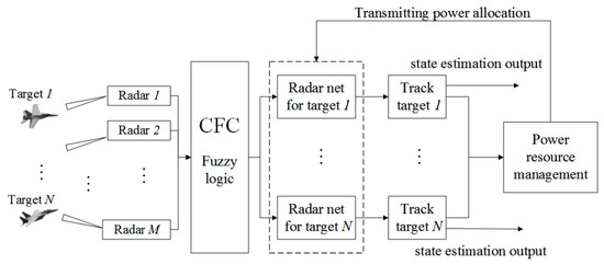
Figure 1.
Radar network resource management process.
2.1. Target Motion Model
Assume that all targets move in a straight line at a constant speed, the expression is as follows:
where denotes the state vector of the target q at the kth sample interval. and represents position and velocity vector of the target, respectively. is a 4 × 4 state transition matrix:
where is second-order identity matrix. is the tracking sample interval, represents the direct product of the matrix. denotes zero mean Gaussian white noise, and its covariance is:
where is the noise intensity [18].
2.2. Measurement Model
Radar obtains target range, azimuth and Doppler information from target echoes. At the kth sample interval, the nonlinear measurement equation of the target q observed by the radar i is:
where
, and are distance, azimuth and Doppler frequency information respectively:
where represents carrier wavelength of radar q. denotes zero-mean Gaussian white noise, and its covariance is:
Where , and represent the measurement variances of distance, azimuth, and Doppler frequency respectively [19], and their expressions are:
where and represent limited bandwidth and time width respectively. represents the zero power beam width of the receiving antenna. c is speed of light. Assuming that there is no deviation between the radar beam irradiation direction and the azimuth of the target q, the expression of the signal-to-noise ratio of the echo of the target q received by the radar i is [16]:
where represents transmit power of the radar i. represents transmit power of the radar i.represents signal strength attenuation along the transmission path.
2.3. Fusion Center
Clustered radars send the measurement information to the fusion center for further processing. At the kth sample interval, the measurement of target q can be obtained from the fusion center:
where , and represent the measurement set of the distance, azimuth, and Doppler frequency information of target q at the kth sample interval respectively., and represent the noise vectors of the radar measurement parameters. The measurement errors of each radar are independent, and the covariance matrix of the measurement noise vector can be expressed as:
where represents diagonal matrix.
3. Radar Cluster
The radar networks based on unmanned cluster can adjust the form of radar networking according to the battlefield environment. This paper uses FLR to reasonably cluster radars at every moment. To ensure that each target is always observed by a fixed number of radars, the algorithm is designed as shown in Figure 2:
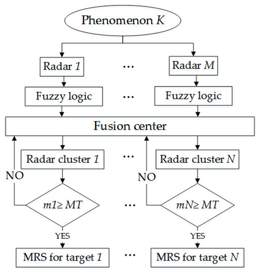
Figure 2.
Flow chart of radar clustering.
Where MT is the preset number of radars that track each target.
3.1. Target Priority Based on Fuzzy Logic Reasoning
FLR is a method for uncertain reasoning problem. It is based on fuzzy logic and uses information such as target attributes and the knowledge base in view of the intuitive and expert considerations to calculate the priority of a target online. The FLR system is shown in Figure 3 [20]:
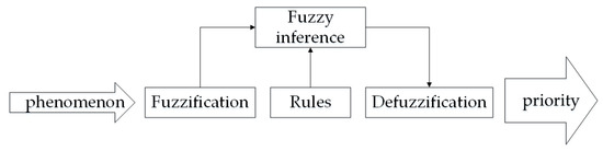
Figure 3.
Flow chart of fuzzy logic reasoning (FLR) system.
3.1.1. Fuzzification
Fuzzification is essentially a concept of map introduced in mathematics, which describes the relationship between the exact numerical value and the fuzzy sets [21]. This paper uses triangular fuzzifier to fuzzify the input numerical value. Its expression is as follows:
where σ is a positive number, whose size is proportional to the anti-interference ability of the triangle fuzzy method. Here we consider three factors that are important to the target as input variables for fuzzy logic reasoning: (1) distance; (2) speed; (3) target identity. The detailed description of these three variables is shown in the Table 1 [22,23].

Table 1.
Fuzzy values related to fuzzy variables.
3.1.2. Fuzzy Rule
The fuzzy rule base provides control rules for fuzzy reasoning, which is related to the distribution of fuzzy values. The more fuzzy the values, the more rules. The form of the fuzzy logic rules in this paper could be represented as:
Based on intuitive and expert considerations, 75 if-then fuzzy rules are obtained, as shown in the Appendix A.
3.1.3. Fuzzy Inference
Firstly, the fuzzy inference needs to match the appropriate rules for the current input value, then use the fuzzy rules to operate on the input value, and finally get the fuzzy output value. According to the Mamdani fuzzy inference method, the fuzzy relation matrix of the ith fuzzy rule can be obtained [24].
where is membership function, is the minimum operator and .
The fuzzy relation R constituted by all fuzzy rules Ri is:
where is the fuzzy union operation, so the conclusion D’ is:
where is the fuzzy intersection operation, and is:
So, the membership function of is:
where is the height of the intersection of the , , and the intersection of, , and , which can be understood as fitness of the ,, and the intersection of , and .
The geometric property of fuzzy inference is to use as the reference cutting set , and then get the conclusion D’. Figure 4 shows the geometric properties of multiple condition fuzzy inference when the number of rules is 2.
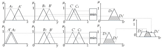
Figure 4.
Three-input two-rule reasoning.
3.1.4. Defuzzification
The results obtained by fuzzy inference are fuzzy, which cannot be used to directly measure the priority of the target. So, the fuzzy value need to convert to the exact numerical value. Defuzzification can be regarded as the mapping of fuzzy space to exact numerical space. This paper uses the center average defuzzifier for defuzzification. In this method, after weighted average, the output numerical value of each element is taken as the execution quantity. Where, the weight is the height of the corresponding fuzzy set [25]. The numerical value calculated by the following formula:
where is the center of mass of the ith fuzzy set, is the maximum membership function of the fuzzy set. is the numerical result calculated by center average defuzzifier, that is, the target priority calculated by the entire FLR.
3.2. Radar Clustering Strategy Based on the Target Priority
The priority of each target for different radar at the kth sample interval is constituted into matrix (M is the number of radar, N is the number of target), then the radars are clustered by the following methods.
- Select the highest priority value from the matrix . Then the radar mk corresponding to is assigned to the radar cluster that will track the target nk. Set all values of the matrix in line mk to zeros.
- Repeat step 1 to assign radars to each target. If the number of radars assigned to a target has reached the preset require number MT, set all values in the column of the target in matrix to 0. Figure 5 shows the flow of radar clustering algorithm.
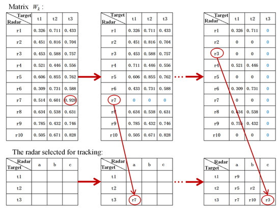 Figure 5. Example of radar assignment process.
By using the above radar-clustering algorithm based on FLR at each sample interval, each radar can track the target with high priority to itself.
4. Management of Power Resource of Radar Networks
In order to deal with the uncertainty of the environment and target information, this paper treats target RCS as uncertainty information. So, the power resource CCP model for multiple-radar tracking multiple-target is constructed. The Bayesian Cramer-Rao low bound (BCRLB) is used to measure the tracking accuracy of the targets. With the radar-clustering algorithm based on FLR proposed in the previous section, the multiple-radar tracking multiple-target system is divided into N (the number of target) multiple-radar tracking single-target subsystems. Then, aiming at the subsystem, the transmitting power CCP submodel for multiple-radar tracking single-target is established. The submodel is solved by the hybrid intelligence algorithm, which is formed by embedding the stochastic simulation into the genetic algorithm.
4.1. BCRLB of Target Tracking
In Bayesian estimation, for the target of a single motion model, the BCRLB matrix provides a lower bound for the MSE of the state estimation of the target [26]:
where, represents the inverse of the BIM matrix, is the expected value of . is the predicted value of the state vector of the target q [27]. is the measurement set of the radar observing the target q. m is the number of radars clustered to observe the target q in the same times.
At the kth sample interval, there are m radars for clustering observation of the target q, so the BIM matrix of the target q is [26]:
The data information matrix is a function of radar transmit power and target RCS . So BIM can be rewritten as:
Reverse the matrix to get the corresponding BCRLB matrix:
The is the functions of parameters such as radar transmit power. Therefore, the following formula could be used as the cost function of target allocation.
4.2. Power Resource Management Opportunity Constraint Programming Model
The purpose of this section is to optimize the transmit power of each radar on the basis of meeting the preset tracking error conditions of each target. The advantage of CCP is that it can avoid some extreme constraints on the detection performance [28]. In practice, the target’s identity, attitude and orientation are uncertain. In this paper, we consider the target’s RCS as a random variable [29]. Therefore, we build the following model:
where, is the confidence level, which represents the probability of the random constraint being established, and is affected by many factors, such as types, attitude and mobility of the target. is the number of radars observed on the target q cluster, M is the total number of radars, and N is the total number of targets, represents the total transmitting power of all radars that have observed target q. is the specified total tracking error threshold. is the transmit power of radar i tracking the target q.
In previous papers, the optimization function of a joint radar node and transmitting power resource management model usually includes two variables: the radar node and the transmitting power. This model is also the same. Solving such multiple variables optimization problems usually requires a large amount of calculation. In order to avoid multiple variables in the optimization function, we designed the above FLR-based radar-clustering algorithm. So the radar node allocation problem is solved online. After radar clustering, the former CCP model can be transformed into:
4.3. Model Solving Method
Embedding stochastic simulation into the genetic algorithm to form a hybrid intelligent algorithm can solve the problem of CCP with a confidence level of , so as to predict the transmit power of each radar in the next sampling period [28].
4.3.1. Stochastic Simulation
Use Algorithm 1 to verify whether the decision vector meets the confidence level a [28].
| Algorithm 1. Stochastic simulation algorithm |
| Step (1): Let . |
| Step (2): Generate N sets of RCS vector samples from sample space . |
| Step (3): If , then . Repeat steps 2 to 3. |
| Step (4): Let . |
| Step (5): If , then satisfies the confidence level , otherwise it does not. |
4.3.2. Hybrid Intelligent Algorithm
At the kth sampling time, the transmit power of the radar at the next time is predicted by Algorithm 2:
| Algorithm 2. Stochastic simulation algorithm |
| Step (1): According to the target motion equation under zero process noise, predict the state vector at the moment;. |
| Step (2): Initialize population S and stain length N, then verify the feasibility of chromosomes using random simulation. |
| Step (3): Hybridize and mutate chromosomes, use random simulation to verify whether the chromosomes meet the constraints, and correct those chromosomes that do not meet the constraints. |
| Step (4): Calculate the objective function value of all chromosomes, and calculate the fitness function value of each stain according to the objective function value. |
| Step (5): Use roulette to select chromosomes. If the requirements of the stopping rules are not met, go to (3). If the stopping rules are met, go to step (6). |
| Step (6): Returns the best chromosome as the optimal radar transmit power . |
5. Target State Estimation
The state vector of the target is estimated from the radar measurement information. Since measurement equations are highly nonlinear, this paper uses Algorithm 3 to predict the state vector of each target.
| Algorithm 3. UKF algorithm |
| Step (1): Let k = 1, initialize each radar transmit power , target state and covariance matrix . |
| Step (2): The transmitting power of each radar is , get the measured value of the target, and calculate . |
| Step (3): Construct the 2L + 1 sigma point set and the weights corresponding to the point set according to the following formula. Where, is a scale factor, represents the ith column of the square root of the matrix; I represents the dimension of the state vector. |
| Step (4): Map the sigma point set to the predicted point set through the state transition function , and calculate the new target state and variance by weighting. |
| Step (5): Map the sigma prediction point set to the new point set through the measurement equation, and calculate the mean , variance and . |
| Step (6): Calculate the gain matrix and update and covariance matrix with the gain matrix. |
| Step (7): According to the intelligent hybrid algorithm proposed above, predict the radar transmission power at the kth moment, let and then jump to step (2) |
6. Simulation Results and Analysis
This section designs a scenario where multiple radars are tracking multiple targets to verify the effectiveness of the above algorithm. In order to simplify the analysis and eliminate the influence of radar deployment on the tracking performance, the positions of the 12 radars in the scene are not changed, and all radars form a square network. There are three targets in the scene, and the starting position of each target is set randomly. The radar parameters of each radar are the same, as shown in the following Table 2.
Table 2.
Parameters of radars.
The position parameters of radars are shown in Table 3:
Table 3.
Position parameters of radars.
The status parameters of the three targets are shown in the Table 4:
Table 4.
State parameter of targets.
The distribution of radar and targets is shown in Figure 6:
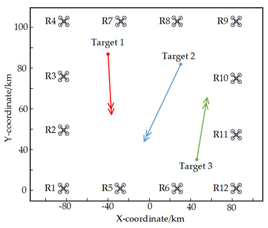
Figure 6.
The distribution of radars and targets.
There are 40 frames in the simulation process. Within each frame, the radar clustering method based on FLR is first used to implement the selection of radar node. Then, the CCP model is used to allocate the transmitting power of each radar.
In order to facilitate comparison, this paper extracts all the numerical results obtained by FLR at each moment and displays them uniformly. So the simulation results of the priority of each target to different radars are shown below:
Figure 7 shows all the numerical solutions obtained by FLR, which can show the change of the priority of the targets for each radar. The value of is between (0,1). The legend on the right shows the correspondence between colors and numerical values of . Warm colors represent higher numerical value , which means the target has a higher priority, while cool tones have the opposite. As the picture shows, target 1 has high priority for radars 2, 3, 4, and 7 at the beginning. As the target 1 moves, its priority for radars 4 and 7 gradually decreases, and for radar 2 it gradually increases. The priority change of target 2 is similar to target 1, first, the priority of target 1 two for radars 8, 9, and 10 is high. As it moves, its priority for radars 5 and 6 gradually increases. The situation of target 3 is slightly different. Because target 3 is closer to radar 11, its priority for radar 11 is always high. So, it can be proved by the simulation results that as the target moves, the targets’ priorities for different radars will change accordingly.
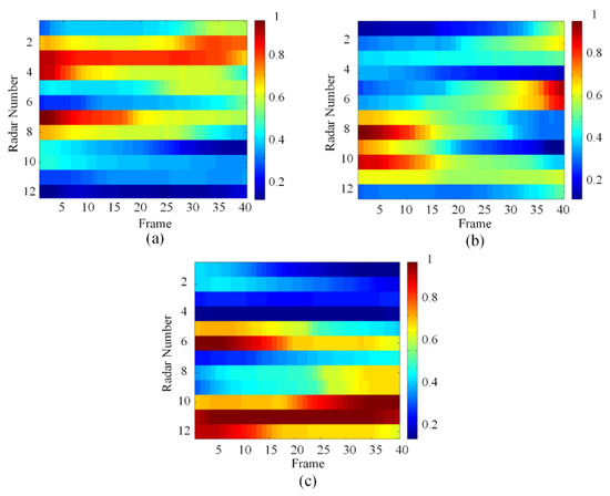
Figure 7.
The priorities of each target: (a) target 1, (b) target 2, and (c) target 3.
According to the above numerical values in Figure 7, using the radar node selection algorithm proposed in Section 3.2, the clustering situation of radar and target at each moment can be obtained.
Figure 8 shows the radar-clustering situation for each target at different time. It can be seen from the figure that each target is always tracked by three radars from different angles. Combining Figure 6 and Figure 8, it can be found that only three radars that are relatively close to the target will cluster and track it at the same time. The number of radars involved in tracking target 2 is the largest during the entire tracking process. This is because target 2 has the fastest speed and the widest area of motion coverage.
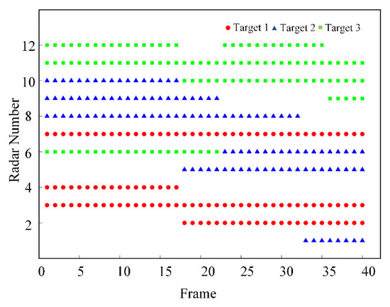
Figure 8.
Radar clustering at each moment.
After obtaining the clustering situation of radars for targets at each moment. The hybrid intelligent algorithm is used to solve the power CCP model for multiple-radar tracking single-target. From this, the total transmitting power of each radar can be obtained.
Figure 9 shows the total power of the radars tracking each target at each moment. Where α is the confidence level. It can be found that as the confidence level α decreases, the transmit power also decreases. When α is reduced by 0.5, the radar can save nearly 9% of the total power. In this article, RCS is set as a random variable, so the transmission power fluctuates randomly following the change of RCS. Comparing the total transmit power of the three targets, it can be found that the total transmit power of target 2 is the highest, and the total transmit power of target 3 is the lowest, which is caused by the distance between the target and the radar. The above simulation results prove that this algorithm can save large transmit power.
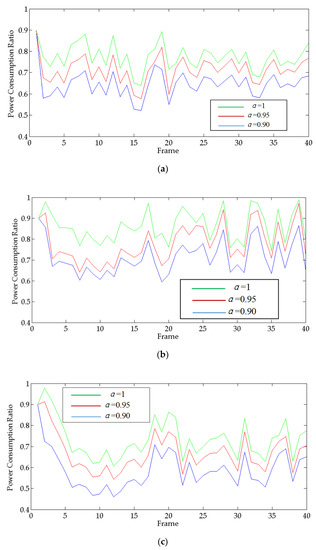
Figure 9.
Total power consumption ratio: (a) Target 1; (b)Target 1; (c)Target 1.
In order to clearly show the distribution of the transmit power for each radar, Figure 10 gives the ratio of the transmitting power of each radar to the total transmitting power when the confidence level α is 0.9.
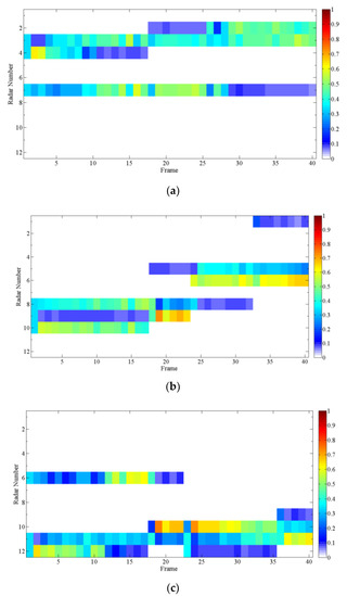
Figure 10.
Percentage of radar transmitting power: (a) Target 1; (b) Target 2; (c) Target 3.
It is found from the three diagrams in Figure 10 that each target is always tracked by three radars, and it is very rare that one radar operates at extremely high power. It proves that the algorithm effectively limits the transmitting power of each radar. The transmitting power of each radar in Figure 10 is in different forms of fluctuations, because each radar observes the target at different angles.
In order to show the tracking performance of the algorithm in this paper, we compare the root mean square error(RMSE) of target tracking error obtained by this algorithm with the RMSE of equal power allocation in Figure 11.
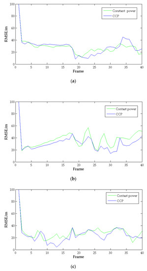
Figure 11.
The RMSE of each target tracking error: (a) Target 1; (b) Target 2; (c) Target 3.
Figure 11 shows the changes in the RMSE of each target tracking error at different times. When α is 0.9, the RMSE obtained by the CCP model is represented by the blue curve. When each radar uses 90% of its own power to track the targets, the RMSE of each target is represented by the green curve. Because of the randomness of the target RCS, the RMSE of both also fluctuate. It can be seen from the Figure 11 that the gap between the blue and green lines of each target is acceptable, which can prove that the algorithm in this paper is in high tracking accuracy while effectively saving power.
7. Conclusions
This paper provides a new solution to the issues of joint radar node selection and power allocation for radar networks based on UAV. An innovative radar-clustering algorithm is proposed to select the radar node online. In the paper, the target RCS is treated as a random variable to ensure the stability of the model in real scenarios. Aiming at the problem that the size of the UAV limits the radar transmitting power, the CCP model is used to optimize radar transmit power. Simulation results show that the algorithm in this paper can reasonably schedule radar node and effectively save the radar power resources.
The future work will be directed to the following aspects: The paper assumes that the position of each drone is fixed. This does not fully take advantage of unmanned cluster. In the future, we can rationally schedule the layout of UAVs based on the target-tracking situation to achieve better tracking performance.
Author Contributions
The work was conducted under the cooperation of all authors. Y.Z. conceived and designed the algorithm and simulations; Q.H. analyzed the data; M.P. verifified the results; Y.Z. wrote the paper; M.P. and Q.H. reviewed the manuscript. All authors have read and agreed to the published version of the manuscript.
Funding
This study is supported by the National Natural Science Foundation of China (Nos. 61671241) and the Aeronautics Science Foundation of China (Grant No. 2017ZC52036).
Conflicts of Interest
The authors declare no conflict of interest.
Appendix A
Based on expert experience and experimental data, 63 if-then rules are listed below:
- IF (range is close) AND (speed is very slow) AND (identity is low risk), then (priority is Medium)
- IF (range is close) AND (speed is very slow) AND (identity is medium risk), then (priority is High)
- IF (range is close) AND (speed is very slow) AND (identity is high risk), then (priority is High)
- IF (range is close) AND (speed is slow) AND (identity is low risk), then (priority is Medium)
- IF (range is close) AND (speed is slow) AND (identity is medium risk), then (priority is High)
- IF (range is close) AND (speed is slow) AND (identity is high risk), then (priority is High)
- IF (range is close) AND (speed is medium) AND (identity is low risk), then (priority is Medium)
- IF (range is close) AND (speed is medium) AND (identity is medium risk), then (priority is High)
- IF (range is close) AND (speed is medium) AND (identity is high risk), then (priority is High)
- IF (range is close) AND (speed is fast) AND (identity is low risk), then (priority is High)
- IF (range is close) AND (speed is fast) AND (identity is medium risk), then (priority is High)
- IF (range is close) AND (speed is fast) AND (identity is high risk), then (priority is High)
- IF (range is close) AND (speed is very fast) AND (identity is low risk), then (priority is High)
- IF (range is close) AND (speed is very fast) AND (identity is medium risk), then (priority is High)
- IF (range is close) AND (speed is very fast) AND (identity is high risk), then (priority is High)
- IF (range is medium-close) AND (speed is very slow) AND (identity is low risk), then (priority is Medium)
- IF (range is medium-close) AND (speed is very slow) AND (identity is medium risk), then (priority is Medium)
- IF (range is medium-close) AND (speed is very slow) AND (identity is high risk), then (priority is Medium)
- IF (range is medium-close) AND (speed is slow) AND (identity is low risk), then (priority is Medium)
- IF (range is medium-close) AND (speed is slow) AND (identity is medium risk), then (priority is Medium)
- IF (range is medium-close) AND (speed is slow) AND (identity is high risk), then (priority is High)
- IF (range is medium-close) AND (speed is medium) AND (identity is low risk), then (priority is Medium)
- IF (range is medium-close) AND (speed is medium) AND (identity is medium risk), then (priority is Medium)
- IF (range is medium-close) AND (speed is medium) AND (identity is high risk), then (priority is High)
- IF (range is medium-close) AND (speed is fast) AND (identity is low risk), then (priority is Medium)
- IF (range is medium-close) AND (speed is fast) AND (identity is medium risk), then (priority is High)
- IF (range is medium-close) AND (speed is fast) AND (identity is high risk), then (priority is High)
- IF (range is medium-close) AND (speed is very fast) AND (identity is low risk), then (priority is Medium)
- IF (range is medium-close) AND (speed is very fast) AND (identity is medium risk), then (priority is High)
- IF (range is medium-close) AND (speed is very fast) AND (identity is high risk), then (priority is High)
- IF (range is medium) AND (speed is very slow) AND (identity is low risk), then (priority is Low)
- IF (range is medium) AND (speed is very slow) AND (identity is medium risk), then (priority is Medium)
- IF (range is medium) AND (speed is very slow) AND (identity is high risk), then (priority is Medium)
- IF (range is medium) AND (speed is slow) AND (identity is low risk), then (priority is Low)
- IF (range is medium) AND (speed is slow) AND (identity is medium risk), then (priority is Medium)
- IF (range is medium) AND (speed is slow) AND (identity is high risk), then (priority is Medium)
- IF (range is medium) AND (speed is medium) AND (identity is low risk), then (priority is Medium)
- IF (range is medium) AND (speed is medium) AND (identity is medium risk), then (priority is Medium)
- IF (range is medium) AND (speed is medium) AND (identity is high risk), then (priority is Medium)
- IF (range is medium) AND (speed is fast) AND (identity is low risk), then (priority is Medium)
- IF (range is medium) AND (speed is fast) AND (identity is medium risk), then (priority is Medium)
- IF (range is medium) AND (speed is fast) AND (identity is high risk), then (priority is High)
- IF (range is medium) AND (speed is very fast) AND (identity is low risk), then (priority is Medium)
- IF (range is medium) AND (speed is very fast) AND (identity is medium risk), then (priority is Medium)
- IF (range is medium) AND (speed is very fast) AND (identity is high risk), then (priority is High)
- IF (range is medium-far) AND (speed is very slow) AND (identity is low risk), then (priority is Low)
- IF (range is medium-far) AND (speed is very slow) AND (identity is medium risk), then (priority is Low)
- IF (range is medium-far) AND (speed is very slow) AND (identity is high risk), then (priority is Medium)
- IF (range is medium-far) AND (speed is slow) AND (identity is low risk), then (priority is Low)
- IF (range is medium-far) AND (speed is slow) AND (identity is medium risk), then (priority is Low)
- IF (range is medium-far) AND (speed is slow) AND (identity is high risk), then (priority is Medium)
- IF (range is medium-far) AND (speed is medium) AND (identity is low risk), then (priority is Low)
- IF (range is medium-far) AND (speed is medium) AND (identity is medium risk), then (priority is Low)
- IF (range is medium-far) AND (speed is medium) AND (identity is high risk), then (priority is Medium)
- IF (range is medium-far) AND (speed is fast) AND (identity is low risk), then (priority is Low)
- IF (range is medium-far) AND (speed is fast) AND (identity is medium risk), then (priority is Medium)
- IF (range is medium-far) AND (speed is fast) AND (identity is high risk), then (priority is Medium)
- IF (range is medium-far) AND (speed is very fast) AND (identity is low risk), then (priority is Low)
- IF (range is medium-far) AND (speed is very fast) AND (identity is medium risk), then (priority is Medium)
- IF (range is medium-far) AND (speed is very fast) AND (identity is high risk), then (priority is Medium)
- IF (range is far) AND (speed is very slow) AND (identity is low risk), then (priority is Low)
- IF (range is far) AND (speed is very slow) AND (identity is medium risk), then (priority is Low)
- IF (range is far) AND (speed is very slow) AND (identity is high risk), then (priority is Medium)
- IF (range is far) AND (speed is slow) AND (identity is low risk), then (priority is Low)
- IF (range is far) AND (speed is slow) AND (identity is medium risk), then (priority is Low)
- IF (range is far) AND (speed is slow) AND (identity is high risk), then (priority is Medium)
- IF (range is far) AND (speed is medium) AND (identity is low risk), then (priority is Low)
- IF (range is far) AND (speed is medium) AND (identity is medium risk), then (priority is Low)
- IF (range is far) AND (speed is medium) AND (identity is high risk), then (priority is Medium)
- IF (range is far) AND (speed is fast) AND (identity is low risk) then (priority is Low)
- IF (range is far) AND (speed is fast) AND (identity is medium risk), then (priority is Low)
- IF (range is far) AND (speed is fast) AND (identity is high risk), then (priority is Medium)
- IF (range is far) AND (speed is very fast) AND (identity is low risk), then (priority is Low)
- IF (range is far) AND (speed is very fast) AND (identity is medium risk), then (priority is Low)
- IF (range is far) AND (speed is very fast) AND (identity is high risk), then (priority is Medium)
References
- Huang, H.; Bai, J.; Zhou, H. Present situation and key technologies of unmanned cooperative operation under intelligent air combat system. Navig. Control. 2019, 18, 15–23. [Google Scholar]
- Jens, K.; Oliver, B.; Delphine, C. UAV detection with MIMO radar. In Proceedings of the 2017 International Radar Symposium (IRS), Prague, Czech Republic, 28–30 June 2017. [Google Scholar]
- Yan, J.; Jiu, B.; Liu, H.; Bao, Z. Joint cluster and power allocation algorithm for multiple targets tracking in multistatic radar systems. J. Electron. Inf. Technol. 2013, 35, 1875–1881. [Google Scholar] [CrossRef]
- Godrich, H.; Petropulu, A.; Poor, H. Sensor selection in distributed multiple-radar architectures for localization: A knapsack problem formulation. IEEE Trans. Signal Process. 2012, 60, 247–260. [Google Scholar] [CrossRef]
- He, Q.; Blum, R.; Godrich, H.; Haimovich, A. Target velocity estimation and antenna placement for MIMO radar with widely separated antennas. IEEE J. Sel. Top. Signal Process. 2010, 4, 79–100. [Google Scholar] [CrossRef]
- Ye, Y.; W, Y.; Kirubarajan, T. Scaled accuracy based power allocation for multi-target tracking with colocated MIMO radars. Signal Process. 2019, 158, 227–240. [Google Scholar]
- Shi, C.; Zhou, J.; Wang, F. LPI based resource management for target tracking in distributed radar network. In Proceedings of the 2016 IEEE Radar Conference, Philadelphia, PA, USA, 2–6 May 2016; pp. 822–826. [Google Scholar]
- Yan, J.; Pu, W.; Zhou, S. Collaborative detection and power allocation framework for target tracking in multiple radar system. Inf. Fusion 2020, 55, 173–183. [Google Scholar] [CrossRef]
- Yan, J.; Liu, H.; Pu, W. Joint beam selection and power allocation for multiple targets tracking in netted collocated MIMO radar system. IEEE Trans. Signal Process. 2016, 64, 6417–6427. [Google Scholar] [CrossRef]
- Andargoli, S.; Malekzadeh, J. Target assignment and power allocation for LPI radar networks. In Proceedings of the International Symposium on Artificial Intelligence and Signal Processing, Mashhad, Iran, 3–5 March 2015; pp. 234–239. [Google Scholar]
- Ma, B.; Chen, H.; Sun, B.; Xiao, H. A joint scheme of antenna selection and power allocation for localization in MIMO radar sensor networks. IEEE Commun. Lett. 2014, 18, 2225–2228. [Google Scholar] [CrossRef]
- Chavali, P.; Nehorai, A. Scheduling and power allocation in a cognitive radar network for multiple-target tracking. IEEE Trans. Signal Process. 2012, 60, 715–729. [Google Scholar] [CrossRef]
- She, J.; Wang, F.; Zhou, J. A novel sensor selection and power allocation algorithm for multiple-target tracking in an LPI radar network. Sensors 2016, 16, 2193. [Google Scholar] [CrossRef] [PubMed]
- Yu, Y.; Petropulu, A. A study on power allocation for widely separated CS-based MIMO radar. SPIE Defense, Security, and Sensing. In Proceedings of the International Society for Optical Engineering, Baltimore, MD, USA, 8 June 2012; p. 8365. [Google Scholar]
- Xie, M.; Yi, W.; Kirubarajan, T.; Kong, L. Joint node selection and power allocation strategy for multi-target tracking in decentralized radar networks. IEEE Trans Signal Process. 2018, 66, 729–743. [Google Scholar] [CrossRef]
- Han, Q.; Pan, M.; Liang, Z. Joint power and beam allocation of opportunistic array radar for multiple target tracking in clutter. Digit. Signal Process. 2018, 78, 136–151. [Google Scholar] [CrossRef]
- Han, Q.; Pan, M.; Gong, S.; Long, W. Resource management of opportunistic digital array radar antenna aperture for pattern synthesis. IET Radar Sonar Navig. 2017, 11, 829–837. [Google Scholar] [CrossRef]
- Lewandowski, W.; Azoubib, J.; Klepczynski, W. GPS: Primary tool for time transfer. Proc. IEEE 1999, 87, 163–172. [Google Scholar] [CrossRef]
- Tichavsky, P.; Muravchik, C.; Nehorai, A. Posterior Cramér-Rao bounds for dscrete-time nonlinear filtering. IEEE Trans. Signal Process. 1998, 46, 1386–1396. [Google Scholar] [CrossRef]
- Mamdani, E. Application of fuzzy logic to approximate reasoning using linguistic synthesis. IEEE Tran. Comput. 1977, 26, 1182–1191. [Google Scholar] [CrossRef]
- Klir, G.; Bo, Y. Fuzzy Sets and Fuzzy Logic Theory and Application; Prentice-Hall International: Upper Saddle River, NJ, USA, 1995; p. 6. [Google Scholar]
- Miranda, S.; Baker, C.; Woodbridge, K. Knowledge-based resource management for multifunction radar. IEEE Signal Process. Mag. 2006, 23, 66–76. [Google Scholar] [CrossRef]
- Miranda, S.; Baker, C.; Woodbridge, K. Fuzzy logic approach for prioritisation of radar tasks and sectors of surveillance in multifunction radar. IET Radar, Sonar Navig. 2007, 1, 131–141. [Google Scholar] [CrossRef]
- Wang, L. A Course in Fuzzy Systems and Control; International Edition; Prentice-Hall International: Upper Saddle River, NJ, USA, 1997; pp. 85–86. [Google Scholar]
- Han, Q.; Pan, M.; Zhang, W. Time resource management of OAR based on fuzzy logic priority for multiple target tracking. J. Syst. Eng. Electron. 2018, 29, 742–755. [Google Scholar]
- Glass, J.; Smith, L. MIMO radar resource allocation using posterior Cramer-Rao lower bounds. In Proceedings of the IEEE Aerospace Conference, Big Sky, MT, USA, 5–12 March 2011. [Google Scholar]
- Ristic, B.; Arulampalam, S.; Gordon, N. Beyond the Kalman Filter: Particle Filters for Tracking Applications; Artech House: Fitchburg, MA, USA, 2004; pp. 68–70. [Google Scholar]
- Liu, B. Theory and Practice of Uncertain Programming, 1st ed.; Tsinghua University Press: Beijing, China, 2003; pp. 88–89. [Google Scholar]
- Skolnik, M. Introduction to Radar System, 3rd ed.; Tata McGraw-Hill Publishing Company Limited: New Delhi, India, 2001; pp. 313–402. [Google Scholar]


© 2020 by the authors. Licensee MDPI, Basel, Switzerland. This article is an open access article distributed under the terms and conditions of the Creative Commons Attribution (CC BY) license (http://creativecommons.org/licenses/by/4.0/).