A High Reliability 3D Scanning Measurement of the Complex Shape Rail Surface of the Electromagnetic Launcher

Abstract
:1. Introduction
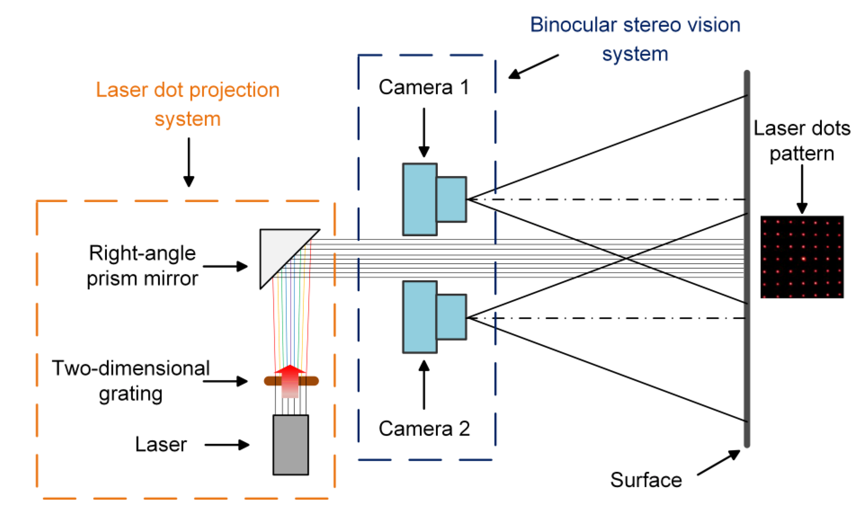
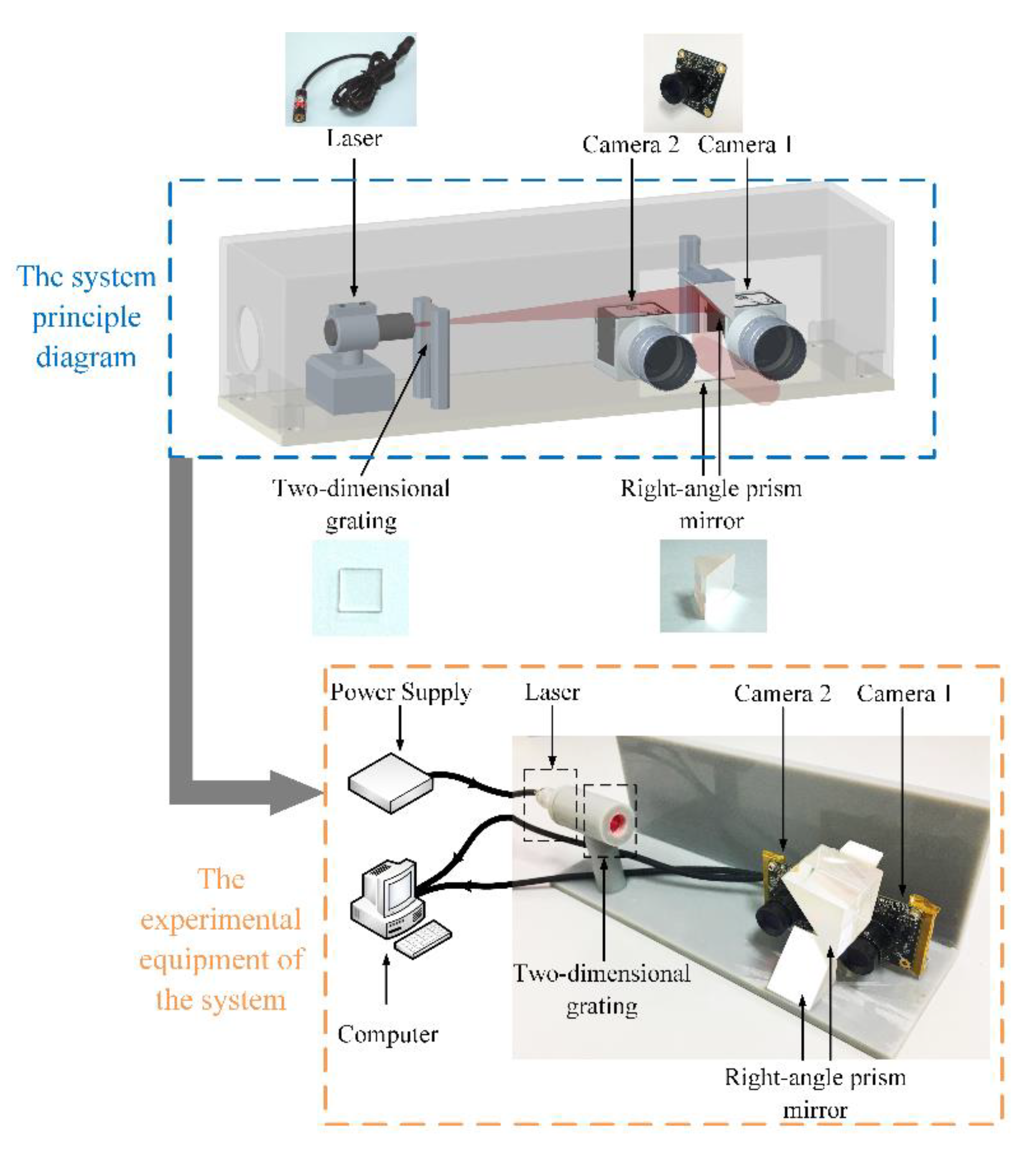
2. Scanning System
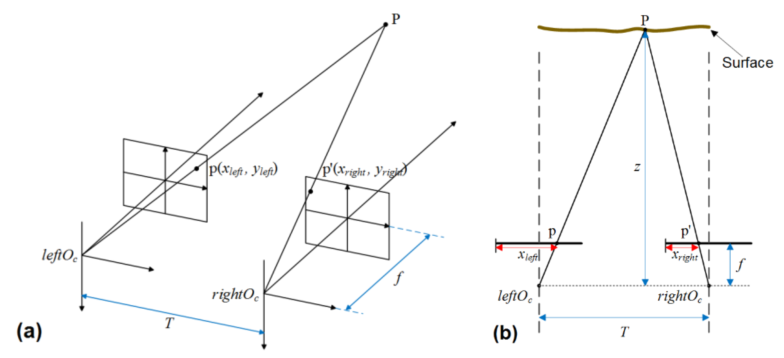
2.1. Binocular Stereo Vision System
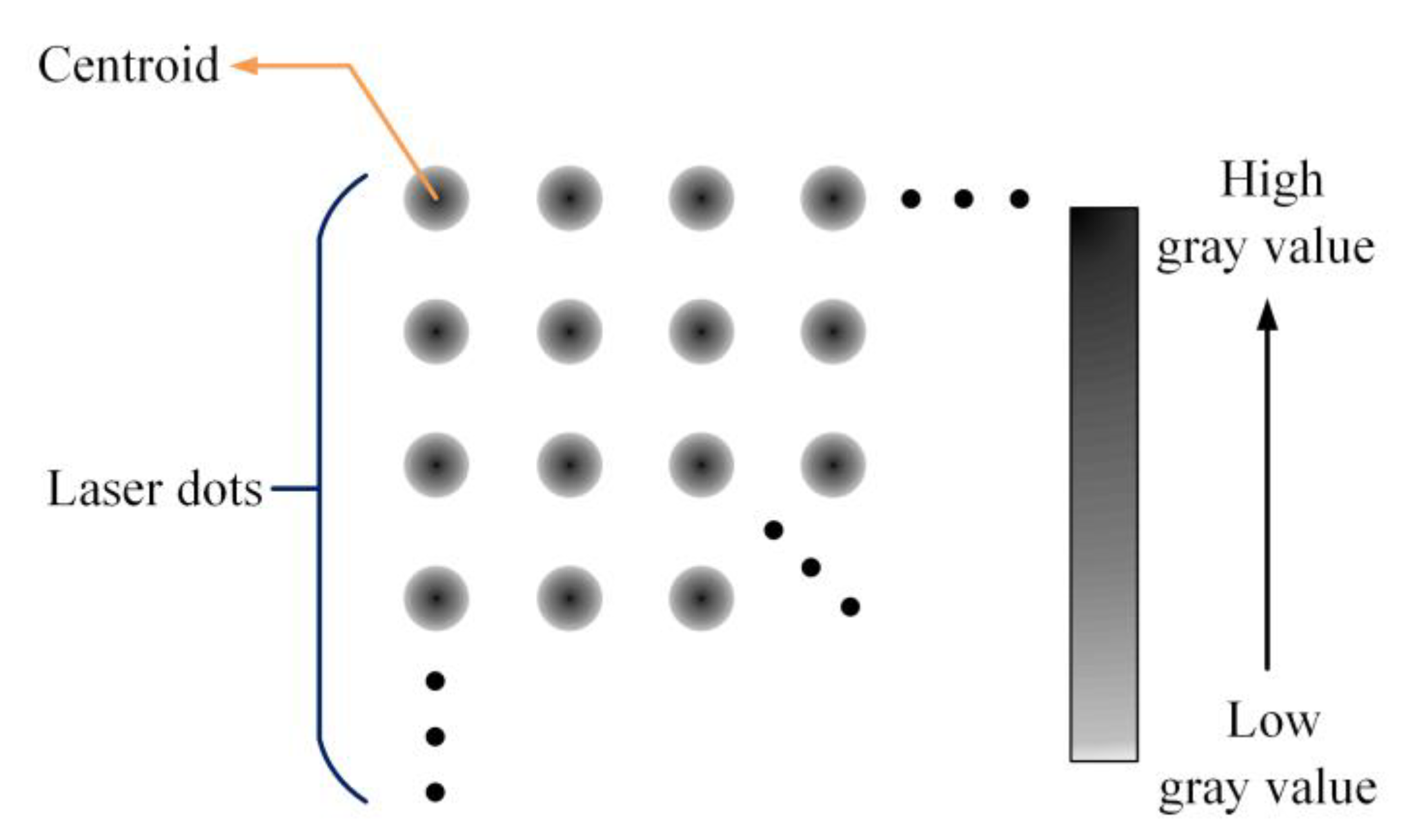
2.2. Laser Dot Projection System
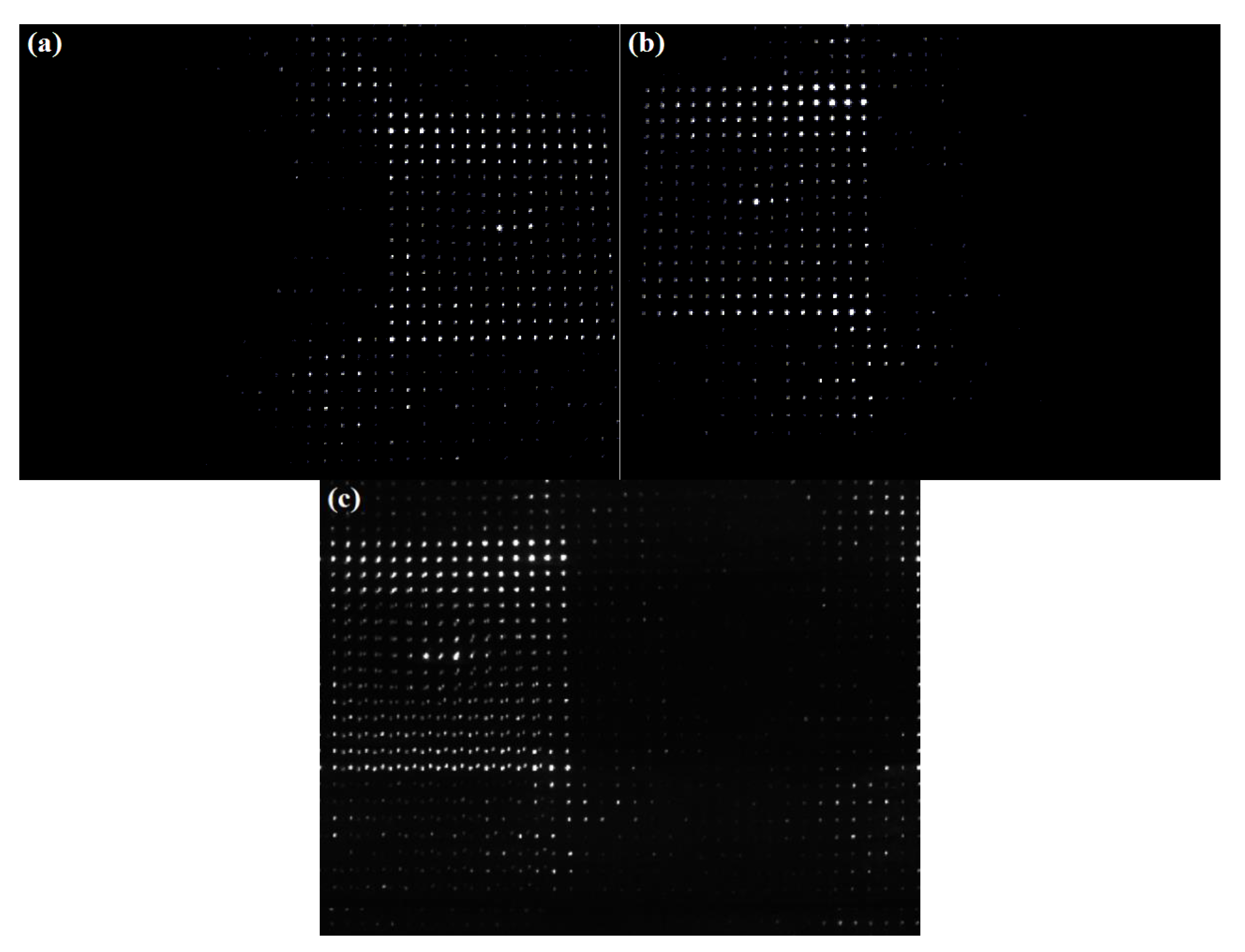
3. High Signal-to-noise Ratio Image Acquisition
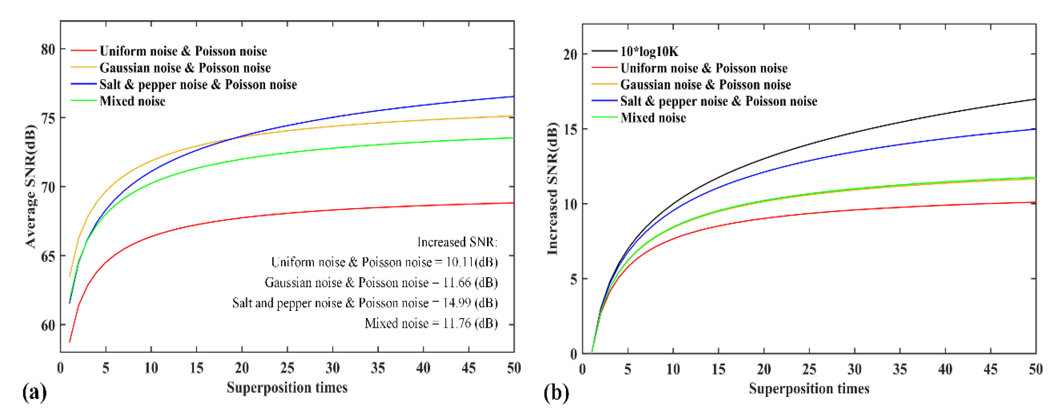
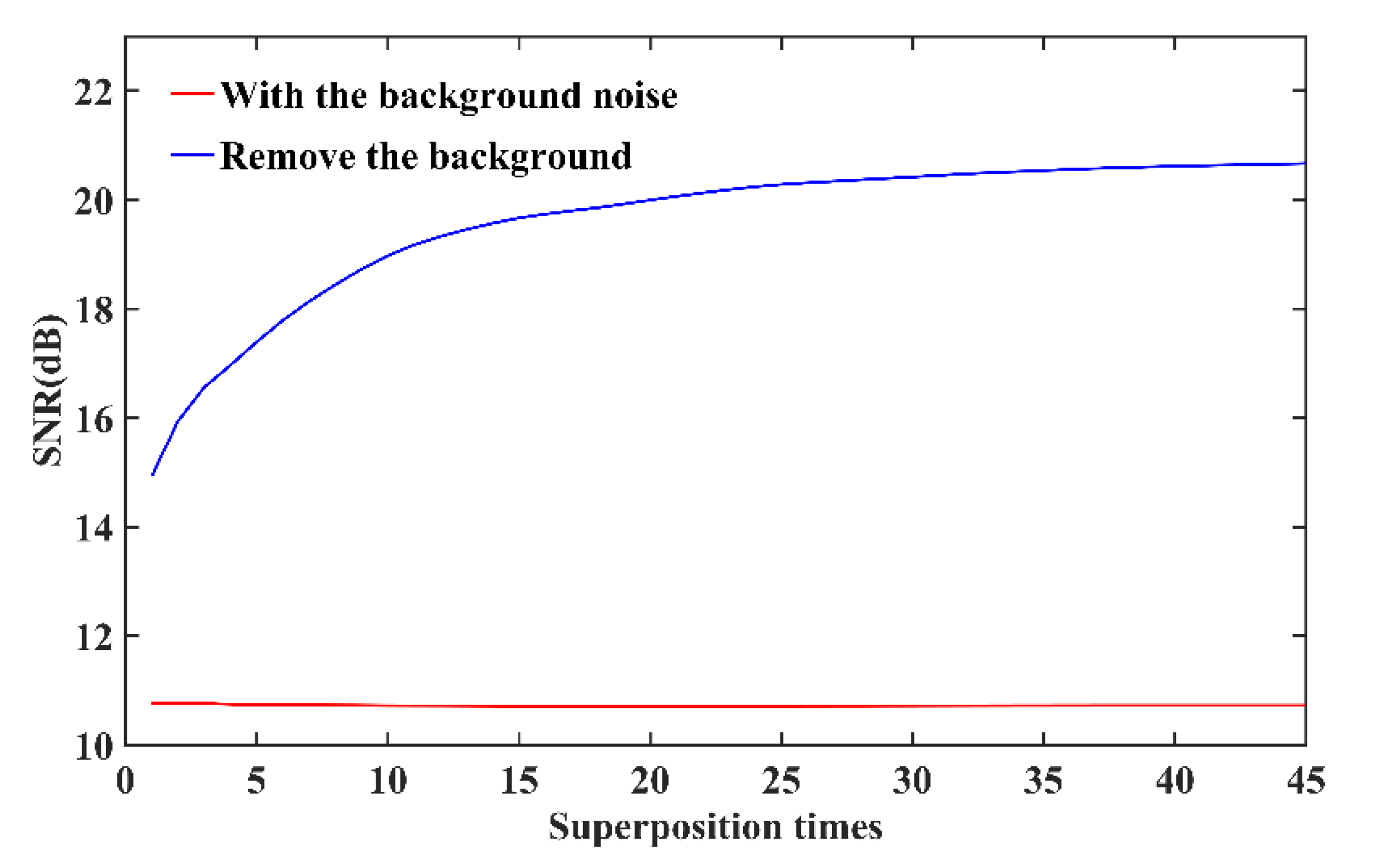
3.1. Image Acquisition Method
3.2. Image Acquisition Experiment
4. Experiment
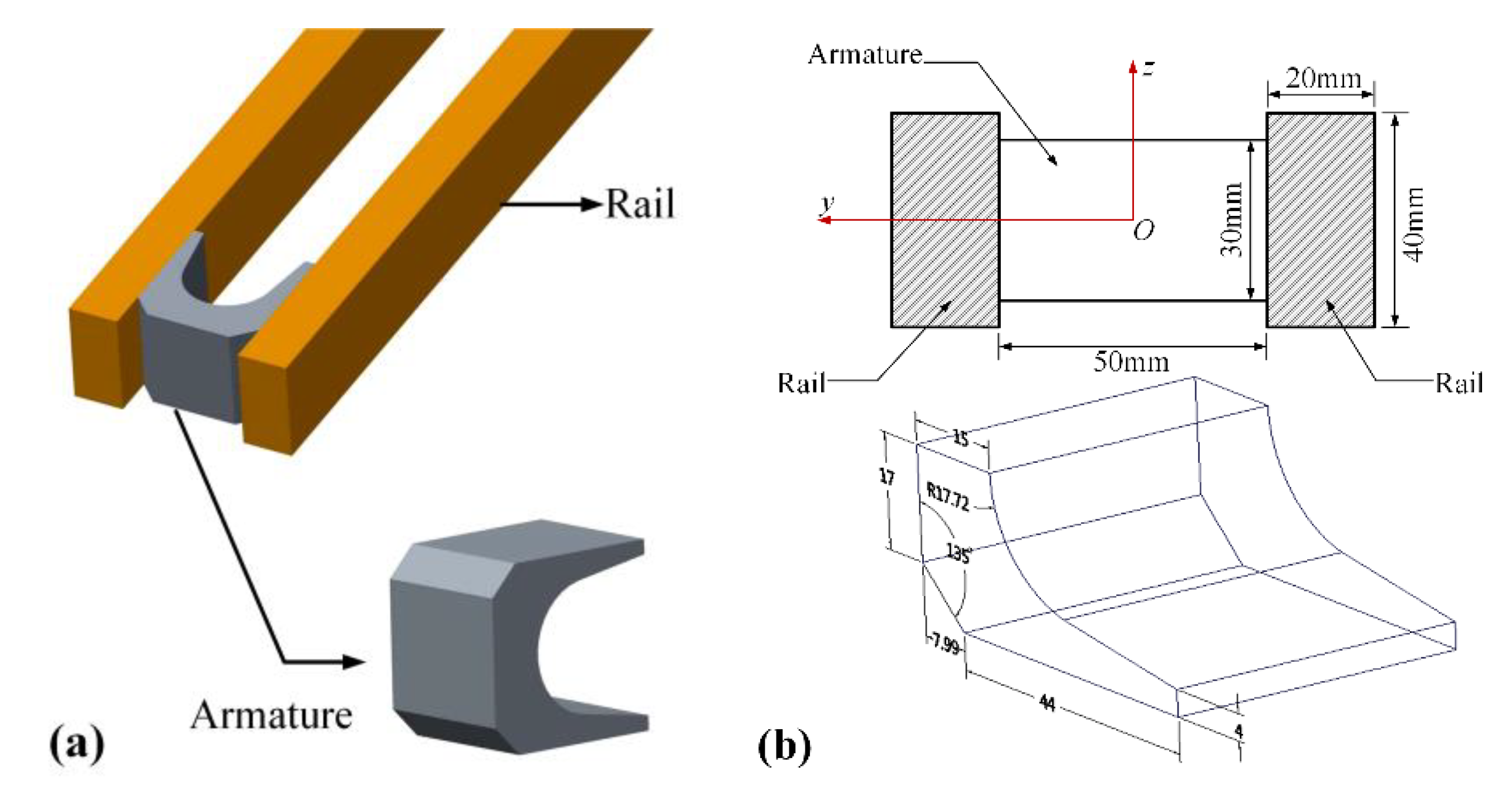
4.1. Experiment System
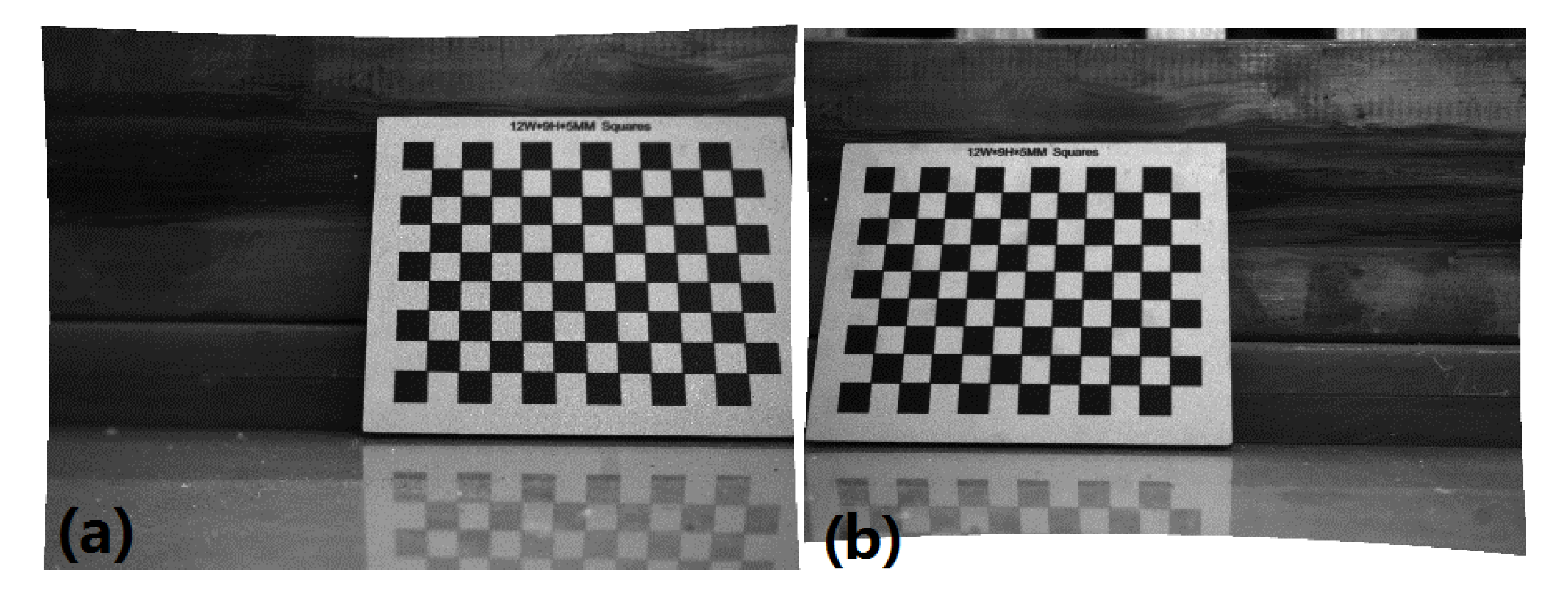
4.2. Stereo Calibration
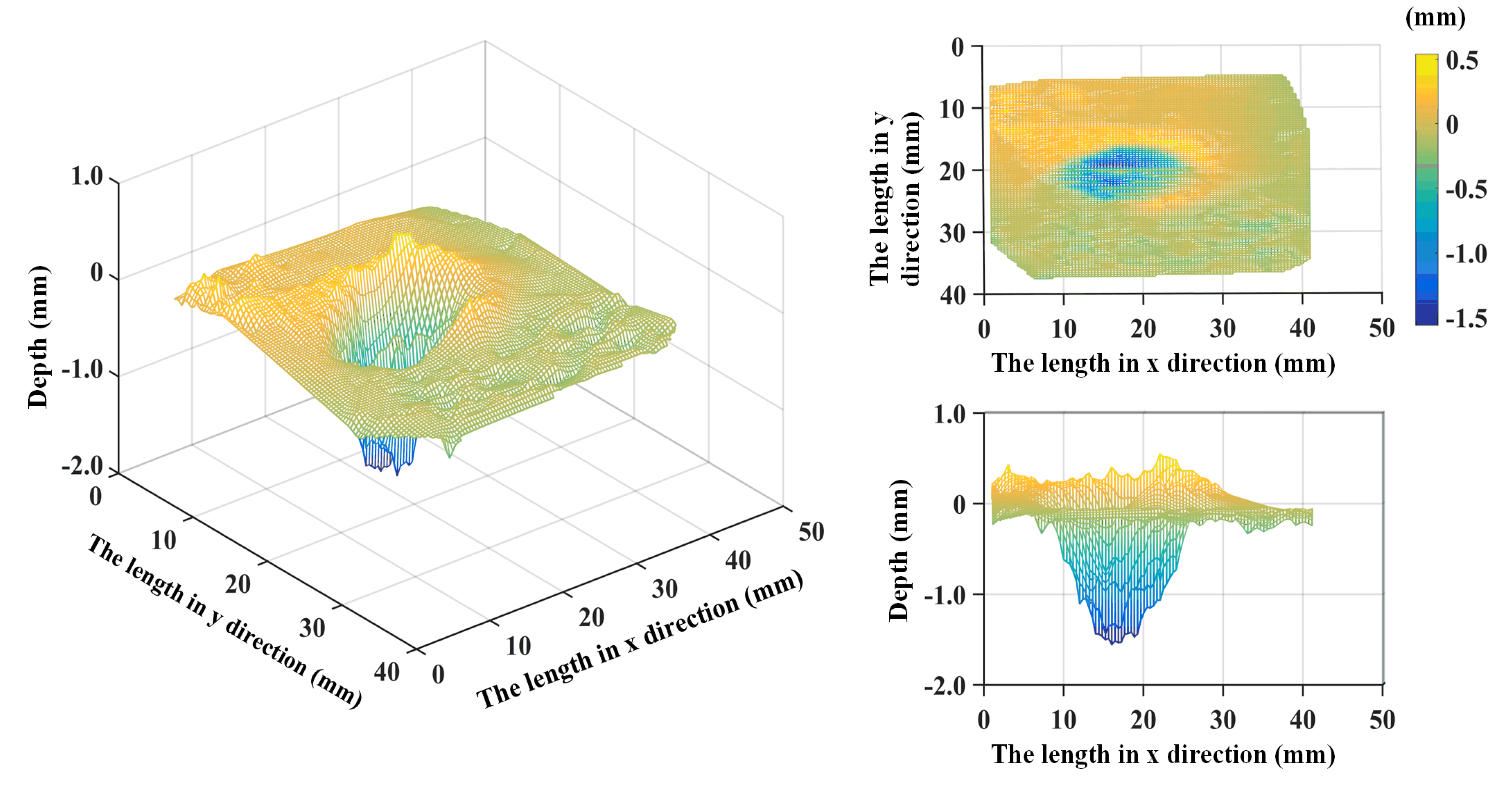
4.3. Result and Discussion
4.4. System Evaluation and Measurement Uncertainty Analysis
4.4.1. System Evaluation
4.4.2. Measurement Uncertainty Analysis
5. Conclusions
Author Contributions
Funding
Conflicts of Interest
References
- Wang, Y.; Marshall, R.A.; Shukang, C. Physics of Electric Launch; Science Press: Beijing, China, 2004. [Google Scholar]
- Persad, C.; Prabhu, G.; White, G.; Yeoh, A.; Eliezer, Z. Characterization of hypervelocity gouge craters in rail conductors. IEEE Trans. Magn. 1997, 33, 401–405. [Google Scholar] [CrossRef]
- Persad, C.; Yeoh, A.; Prabhu, G.; White, G.; Eliezer, Z. On the nature of the armature-rail interface: Liquid metal effects. IEEE Trans. Magn. 1997, 33, 140–145. [Google Scholar] [CrossRef]
- Meger, R.A.; Cooper, K.; Jones, H.; Neri, J.; Qadri, S.; Singer, I.L.; Sprague, J.; Wahl, K.J. Analysis of rail surfaces from a multishot railgun. IEEE Trans. Magn. 2005, 41, 211–213. [Google Scholar] [CrossRef]
- Bair, S.; Cowan, R.; Kennedy, G.; Neu, R.; Siopis, M.; Streator, J.; Thadhani, N. A Survey of Railgun Research at the Georgia Institute of Technology (USA). In Proceedings of the 16th International Symposium on Electromagnetic Launch Technology, Beijing, China, 15–19 May 2012; IEEE: Piscataway, NJ, USA, 2012. [Google Scholar]
- Watt, T.; Stefani, F. The Effect of Current and Speed on Perimeter Erosion in Recovered Armatures. In Proceedings of the 12th Symposium on Electromagnetic Launch Technology, Snowbird, UT, USA, 25–28 May 2004; IEEE: Piscataway, NJ, USA, 2005. [Google Scholar]
- Watt, T.; Stefani, F.; Crawford, M.; Mark, H.; Parker, J. Investigation of damage to solid-armature railguns at startup. IEEE Trans. Magn. 2007, 43, 214–218. [Google Scholar] [CrossRef]
- Zielinski, A.; Watt, T.; Motes, D. Disrupting armature ejecta and its effects on rail damage in solid-armature railguns. IEEE Trans. Plasma Sci. 2011, 39, 941–946. [Google Scholar] [CrossRef]
- Valkenburg, R.J.; McIvor, A.M. Accurate 3D measurement using a structured light system. Int. Soc. Opt. Eng. 1998, 16, 99–110. [Google Scholar] [CrossRef]
- Ishii, I.; Yamamoto, K.; Doi, K.; Tsuji, T. High-Speed 3D Image Acquisition Using Coded Structured Light Projection. In Proceedings of the 2007 IEEE/RSJ International Conference on Intelligent Robots and Systems, San Diego, CA, USA, 29 October–2 November 2007; IEEE: Piscataway, NJ, USA, 2007; pp. 925–930. [Google Scholar]
- Huang, P.S.; Zhang, S. Fast three-step phase-shifting algorithm. Appl. Opt. 2002, 41, 5086–5091. [Google Scholar] [CrossRef] [PubMed]
- Zhang, S.; Yau, S.T. High-resolution, real-time 3D absolute coordinate measurement based on a phase-shifting method. Opt. Express 2006, 14, 2644–2649. [Google Scholar] [CrossRef] [PubMed]
- Takeda, M.; Motoh, K. Fourier transform profilometry for the automatic measurement of 3-D object shapes. Appl. Opt. 1983, 22, 3977–3982. [Google Scholar] [CrossRef] [PubMed]
- Su, X.; Chen, W. Fourier transform profilometry: A review. Opt. Lasers Eng. 2001, 35, 263–284. [Google Scholar] [CrossRef]
- Geng, J. Structured-light 3D surface imaging: A tutorial. Adv. Opt. Photonics 2011, 3, 128–160. [Google Scholar] [CrossRef]
- Howard, I.P.; Rogers, B.J. Binocular Vision and Stereopsis; Oxford University Press: New York, NY, USA, 1995. [Google Scholar]
- Chen, S.; Palmer, A.W.; Grattan, K.T.V.; Meggitt, B.T. Fringe order identification in optical fibre white-light interferometry using centroid algorithm method. Electron. Lett. 1992, 28, 553–555. [Google Scholar] [CrossRef]
- Zhang, Z. A Flexible New Technique for Camera Calibration. IEEE Trans. Pattern Anal. Mach. Intell. 2000, 22, 1330–1334. [Google Scholar] [CrossRef] [Green Version]
- Zhang, Z. Flexible Camera Calibration by Viewing a Plane from Unknown Orientations. In Proceedings of the Seventh IEEE International Conference on Computer Vision, Kerkyra, Greece, 20–27 September 1999; IEEE: Piscataway, NJ, USA, 1999. [Google Scholar]
- Heikkila, J.; Silven, O. A Four-step Camera Calibration Procedure with Implicit Image Correction. In Proceedings of the 1997 IEEE Computer Society Conference on Computer Vision and Pattern Recognition, Oulu, Finland, 17–19 June 1997; IEEE: Piscataway, NJ, USA, 1997. [Google Scholar]
- Camera Calibration Toolbox for Matlab. Available online: http://www.vision.caltech.edu/bouguetj/calib_doc/ (accessed on 11 January 2020).
- Wang, Z.; Yue, J.; Han, J.; Jin, Y.; Li, B. Regional fuzzy binocular stereo matching algorithm based on global correlation coding for 3D measurement of rail surface. Optik 2020, 207, 164488. [Google Scholar] [CrossRef]
- Luhmann, T.; Robson, S.; Kyle, S.; Boehm, J. Close-Range Photogrammetry and 3D Imaging; De Gruyter: Oldenburg, Germany; London, UK, 2013. [Google Scholar]


| Internal Parameters | Left Camera | Right Camera |
|---|---|---|
| αx | 3807.64 ± 26 | 3774.53 ± 22 |
| αy | 3806.41 ± 25 | 3768.74 ± 20 |
| x0 | 1360.88 ± 27 | 1266.53 ± 26 |
| y0 | 897.44 ± 23 | 931.05 ± 21 |
| ac | 0.00 ± 0.00 | 0.00 ± 0.00 |
| k1 | −0.40 ± 0.037 | −0.31 ± 0.032 |
| k2 | 0.45 ± 0.19 | −0.22 ± 0.14 |
| k3 | 0.0080 ± 0.0015 | 0.0020 ± 0.0012 |
| k4 | −0.0037 ± 0.0030 | 0.0023 ± 0.0028 |
| k5 | 0.00 ± 0.00 | 0.00 ± 0.00 |
| External Parameters | X Direction | Y Direction | Z Direction |
|---|---|---|---|
| Rotation vector | −0.03963 | −0.03602 | −0.01476 |
| Translation vector | −39.15007 | 0.63651 | −0.16640 |
| Number of Measurement Times | Measurement Value (mm) | Number of the Step i | Each STEP’ s Value xi (mm) | Average of Each Step’s Value (mm) | Residual (mm) |
|---|---|---|---|---|---|
| 1 | 1.1398 | 0.9976 | |||
| 2 | 2.1749 | 1 | 1.0351 | 0.0375 | |
| 3 | 3.1308 | 2 | 0.9559 | −0.0417 | |
| 4 | 4.1411 | 3 | 1.0103 | 0.0127 | |
| 5 | 5.1062 | 4 | 0.9651 | −0.0325 | |
| 6 | 6.1426 | 5 | 1.0364 | 0.0388 | |
| 7 | 7.1221 | 6 | 0.9795 | −0.0181 | |
| 8 | 8.1232 | 7 | 1.0011 | 0.0035 |
© 2020 by the authors. Licensee MDPI, Basel, Switzerland. This article is an open access article distributed under the terms and conditions of the Creative Commons Attribution (CC BY) license (http://creativecommons.org/licenses/by/4.0/).
Share and Cite
Wang, Z.; Li, B. A High Reliability 3D Scanning Measurement of the Complex Shape Rail Surface of the Electromagnetic Launcher. Sensors 2020, 20, 1485. https://doi.org/10.3390/s20051485
Wang Z, Li B. A High Reliability 3D Scanning Measurement of the Complex Shape Rail Surface of the Electromagnetic Launcher. Sensors. 2020; 20(5):1485. https://doi.org/10.3390/s20051485
Chicago/Turabian StyleWang, Zhaoxin, and Baoming Li. 2020. "A High Reliability 3D Scanning Measurement of the Complex Shape Rail Surface of the Electromagnetic Launcher" Sensors 20, no. 5: 1485. https://doi.org/10.3390/s20051485