Figure 1.
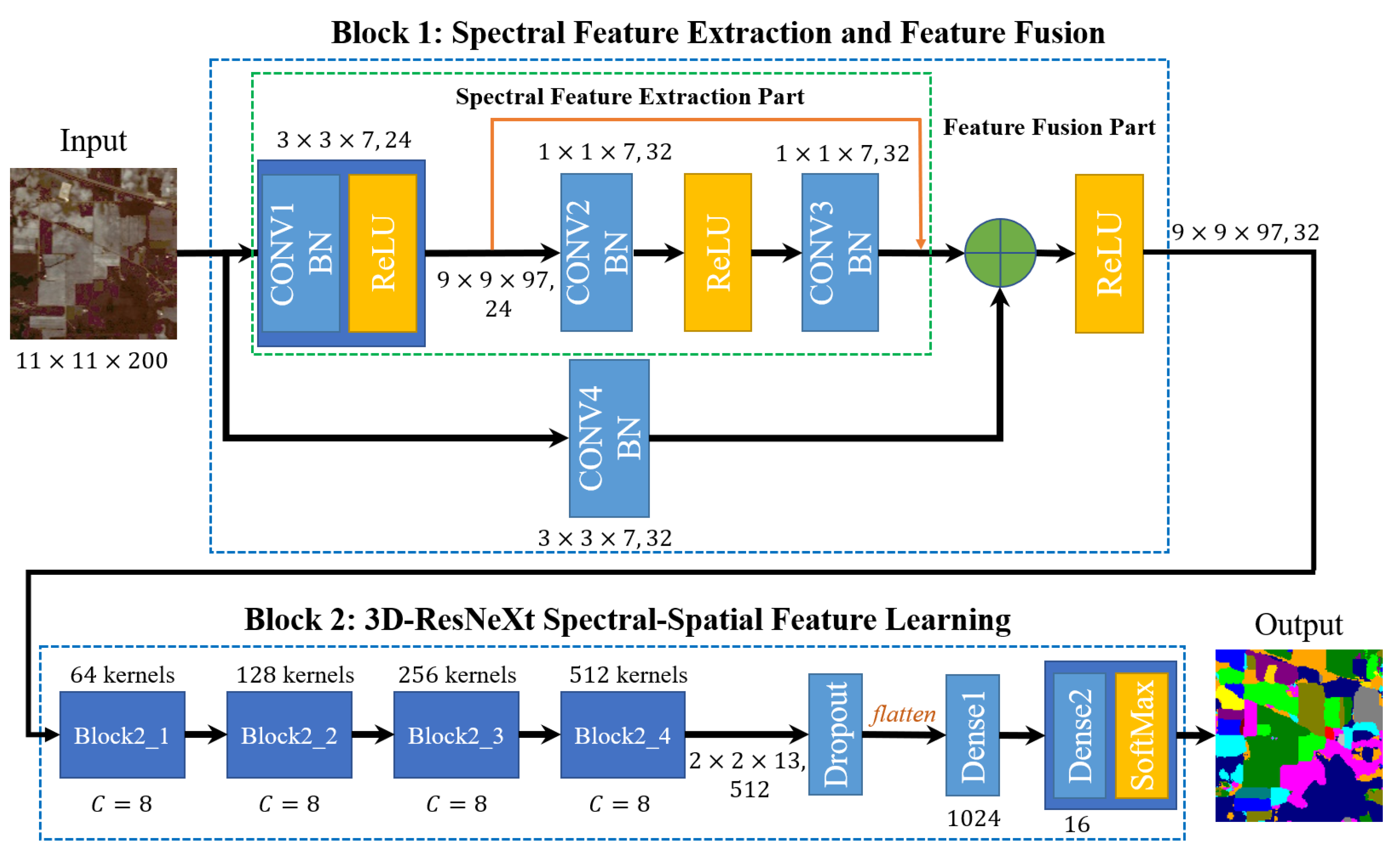
Overall structure of the proposed Hyperspectral Image (HSI) classification framework.
Figure 1.
Overall structure of the proposed Hyperspectral Image (HSI) classification framework.
Figure 2.
The end-to-end HSI classification flowchart.
Figure 2.
The end-to-end HSI classification flowchart.
Figure 3.
Three-dimensional spectral residual block to extract spectral features.
Figure 3.
Three-dimensional spectral residual block to extract spectral features.
Figure 4.
A block of ResNet (Left) and ResNeXt with cardinality = 8 (Right). A layer is shown as (# in channels, filter size, # out channels).
Figure 4.
A block of ResNet (Left) and ResNeXt with cardinality = 8 (Right). A layer is shown as (# in channels, filter size, # out channels).
Figure 5.
General structure of a ResNeXt block with cardinality = 8 (Taking the Block2_1 for example).
Figure 5.
General structure of a ResNeXt block with cardinality = 8 (Taking the Block2_1 for example).
Figure 6.
Precision, Recall, and F1-Score indicators of classes with the smallest number of samples under different training ratios in the three HSI datasets. (Class 9 Oats for IN dataset, Class 9 Shadows for UP dataset, and Class 7 Swamp for KSC dataset).
Figure 6.
Precision, Recall, and F1-Score indicators of classes with the smallest number of samples under different training ratios in the three HSI datasets. (Class 9 Oats for IN dataset, Class 9 Shadows for UP dataset, and Class 7 Swamp for KSC dataset).
Figure 7.
Precision, Recall, and F1-Score indicators of classes with the smallest number of samples under different input spatial size in the three HSI datasets. (Class 9 Oats for IN dataset, Class 9 Shadows for UP dataset, and Class 7 Swamp for KSC dataset).
Figure 7.
Precision, Recall, and F1-Score indicators of classes with the smallest number of samples under different input spatial size in the three HSI datasets. (Class 9 Oats for IN dataset, Class 9 Shadows for UP dataset, and Class 7 Swamp for KSC dataset).
Figure 8.
Precision, Recall, and F1-Score indicators of classes with the smallest number of samples under different cardinality in the three HSI datasets. (Class 9 Oats for IN dataset, Class 9 Shadows for UP dataset, and Class 7 Swamp for KSC dataset).
Figure 8.
Precision, Recall, and F1-Score indicators of classes with the smallest number of samples under different cardinality in the three HSI datasets. (Class 9 Oats for IN dataset, Class 9 Shadows for UP dataset, and Class 7 Swamp for KSC dataset).
Figure 9.
Precision, Recall, and F1-Score indicators of classes with the smallest number of samples of four models using 3-D Convolutional Neural Network (CNN) in the three HSI datasets. (Class 9 Oats for IN dataset, Class 9 Shadows for UP dataset, and Class 7 Swamp for KSC dataset).
Figure 9.
Precision, Recall, and F1-Score indicators of classes with the smallest number of samples of four models using 3-D Convolutional Neural Network (CNN) in the three HSI datasets. (Class 9 Oats for IN dataset, Class 9 Shadows for UP dataset, and Class 7 Swamp for KSC dataset).
Figure 10.
Classification results of the models in comparison for the IN dataset. (a) False color image, (b) Ground-truth labels, (c)–(f) Classification results of 3D-CNN, SSRN, 3D-ResNet, and 3D-ResNeXt.
Figure 10.
Classification results of the models in comparison for the IN dataset. (a) False color image, (b) Ground-truth labels, (c)–(f) Classification results of 3D-CNN, SSRN, 3D-ResNet, and 3D-ResNeXt.
Figure 11.
Classification results of the models in comparison for the UP dataset. (a) False color image, (b) Ground-truth labels, (c)–(f) Classification results of 3D-CNN, SSRN, 3D-ResNet, and 3D-ResNeXt.
Figure 11.
Classification results of the models in comparison for the UP dataset. (a) False color image, (b) Ground-truth labels, (c)–(f) Classification results of 3D-CNN, SSRN, 3D-ResNet, and 3D-ResNeXt.
Figure 12.
Classification results of the models in comparison for the KSC dataset. (a) False color image, (b) Ground-truth labels, (c)–(f) Classification results of 3D-CNN, SSRN, 3D-ResNet, and 3D-ResNeXt.
Figure 12.
Classification results of the models in comparison for the KSC dataset. (a) False color image, (b) Ground-truth labels, (c)–(f) Classification results of 3D-CNN, SSRN, 3D-ResNet, and 3D-ResNeXt.
Figure 13.
The OA and loss of models with different loss functions for the IN dataset, (a) the original cross-entropy loss function, (b) the cross-entropy loss function modified by label smoothing strategy.
Figure 13.
The OA and loss of models with different loss functions for the IN dataset, (a) the original cross-entropy loss function, (b) the cross-entropy loss function modified by label smoothing strategy.
Figure 14.
The OA and loss of models with different loss functions for the UP dataset, (a) the original cross-entropy loss function, (b) the cross-entropy loss function modified by label smoothing strategy.
Figure 14.
The OA and loss of models with different loss functions for the UP dataset, (a) the original cross-entropy loss function, (b) the cross-entropy loss function modified by label smoothing strategy.
Figure 15.
The OA and loss of models with different loss functions for the KSC dataset, (a) the original cross-entropy loss function, (b) the cross-entropy loss function modified by label smoothing strategy.
Figure 15.
The OA and loss of models with different loss functions for the KSC dataset, (a) the original cross-entropy loss function, (b) the cross-entropy loss function modified by label smoothing strategy.
Figure 16.
Precision, Recall, and F1-Score indicators of classes with the smallest number of samples with different loss functions in the three HSI datasets. (Class 9 Oats for IN dataset, Class 9 Shadows for UP dataset, and Class 7 Swamp for KSC dataset).
Figure 16.
Precision, Recall, and F1-Score indicators of classes with the smallest number of samples with different loss functions in the three HSI datasets. (Class 9 Oats for IN dataset, Class 9 Shadows for UP dataset, and Class 7 Swamp for KSC dataset).
Figure 17.
OAs of the 3D-ResNet and 3D-ResNeXt with different ratios of training samples for the IN dataset.
Figure 17.
OAs of the 3D-ResNet and 3D-ResNeXt with different ratios of training samples for the IN dataset.
Figure 18.
OAs of the 3D-ResNet and 3D-ResNeXt with different ratios of training samples for the UP dataset.
Figure 18.
OAs of the 3D-ResNet and 3D-ResNeXt with different ratios of training samples for the UP dataset.
Figure 19.
OAs of the 3D-ResNet and 3D-ResNeXt with different ratios of training samples for the KSC dataset.
Figure 19.
OAs of the 3D-ResNet and 3D-ResNeXt with different ratios of training samples for the KSC dataset.
Table 1.
Numbers of samples of the IN dataset.
Table 1.
Numbers of samples of the IN dataset.
| No. | Class | No. of Samples |
|---|
| 1 | Alfalfa | 46 |
| 2 | Corn-notill | 1428 |
| 3 | Corn-mintill | 830 |
| 4 | Corn | 237 |
| 5 | Grass-pasture | 483 |
| 6 | Grass-trees | 730 |
| 7 | Grass-pasture-mowed | 28 |
| 8 | Hay-windrowed | 478 |
| 9 | Oats | 20 |
| 10 | Soybean-notill | 972 |
| 11 | Soybean-mintill | 2455 |
| 12 | Soybean-clean | 593 |
| 13 | Wheat | 205 |
| 14 | Woods | 1265 |
| 15 | Buildings-Grass-Trees-Drives | 386 |
| 16 | Stone-Steel-Towers | 93 |
| Total | | 10249 |
Table 2.
Numbers of samples of the UP dataset.
Table 2.
Numbers of samples of the UP dataset.
| No. | Class | No. of Samples |
|---|
| 1 | Asphalt | 6631 |
| 2 | Meadows | 18649 |
| 3 | Gravel | 2099 |
| 4 | Trees | 3064 |
| 5 | Painted metal sheets | 1345 |
| 6 | Bare Soil | 5029 |
| 7 | Bitumen | 1330 |
| 8 | Self-Blocking Bricks | 3682 |
| 9 | Shadows | 947 |
| Total | | 42776 |
Table 3.
Numbers of samples of the KSC dataset.
Table 3.
Numbers of samples of the KSC dataset.
| No. | Class | No. of Samples |
|---|
| 1 | Scrub | 761 |
| 2 | Willow swamp | 243 |
| 3 | CP hammock | 256 |
| 4 | Slash pine | 252 |
| 5 | Oak/Broadleaf | 161 |
| 6 | Hardwood | 229 |
| 7 | Swamp | 105 |
| 8 | Graminoid marsh | 431 |
| 9 | Spartina marsh | 520 |
| 10 | Cattail marsh | 404 |
| 11 | Salt marsh | 419 |
| 12 | Mud flats | 503 |
| 13 | Water | 927 |
| Total | | 5211 |
Table 4.
The architecture of the proposed network.
Table 4.
The architecture of the proposed network.
| Layer | Output Size | 3D-ResNeXt | Connected to |
|---|
| Input | | | |
| CONV1 | |
| Input |
| CONV2 | |
same | CONV1 |
| CONV3 | |
same | CONV2 |
| CONV4 | | | Input |
| Add | | | CONV3, CONV4 |
| Block2_1 | |
same | Add |
| Block2_2 | |
| Block2_1 |
| Block2_3 | |
| Block2_2 |
| Block2_4 | |
| Block2_3 |
| Flatten | 26624 | | Block2_4 |
| Dense1 | 1024 | 1024 | Flatten |
| Dense2(SoftMax) | 16 | 16 | Dense1 |
Table 5.
Training time, test time, and OA under different training dataset ratios on the IN dataset by the proposed method.
Table 5.
Training time, test time, and OA under different training dataset ratios on the IN dataset by the proposed method.
| Ratios | Training Time (s) | Test Time (s) | OA (%) |
|---|
| 2:1:7 | 2751.91 | 24.05 | 99.22 |
| 3:1:6 | 3140.21 | 20.88 | 99.82 |
| 4:1:5 | 2709.78 | 17.41 | 99.90 |
| 5:1:4 | 3977.16 | 14.86 | 99.96 |
Table 6.
Training time, test time, and OA under different training dataset ratios on the UP dataset by the proposed method.
Table 6.
Training time, test time, and OA under different training dataset ratios on the UP dataset by the proposed method.
| Ratios | Training Time (s) | Test Time (s) | OA (%) |
|---|
| 2:1:7 | 6077.30 | 54.85 | 99.93 |
| 3:1:6 | 7095.93 | 52.18 | 99.98 |
| 4:1:5 | 6857.42 | 39.32 | 99.99 |
| 5:1:4 | 8630.59 | 40.39 | 99.99 |
Table 7.
Training time, test time, and OA under different training dataset ratios on the KSC dataset by the proposed method.
Table 7.
Training time, test time, and OA under different training dataset ratios on the KSC dataset by the proposed method.
| Ratios | Training Time (s) | Test Time (s) | OA (%) |
|---|
| 2:1:7 | 1260.70 | 10.27 | 99.53 |
| 3:1:6 | 1384.68 | 8.66 | 99.90 |
| 4:1:5 | 1352.76 | 7.25 | 99.96 |
| 5:1:4 | 1656.15 | 5.88 | 99.99 |
Table 8.
Training time, test time, and OA for different input spatial sizes on the IN dataset by the proposed method.
Table 8.
Training time, test time, and OA for different input spatial sizes on the IN dataset by the proposed method.
| Spatial Size | Training Time (s) | Test Time (s) | OA (%) |
|---|
| 7×7 | 1503.56 | 5.38 | 99.90 |
| 9×9 | 2173.70 | 8.75 | 99.90 |
| 11×11 | 3977.16 | 14.86 | 99.96 |
| 13×13 | 4721.14 | 19.41 | 99.95 |
| 15×15 | 6034.21 | 23.28 | 99.90 |
Table 9.
Training time, test time, and OA for different input spatial sizes on the UP dataset by the proposed method.
Table 9.
Training time, test time, and OA for different input spatial sizes on the UP dataset by the proposed method.
| Spatial Size | Training Time (s) | Test Time (s) | OA (%) |
|---|
| 7×7 | 3230.44 | 18.43 | 99.93 |
| 9×9 | 4432.76 | 25.46 | 99.95 |
| 11×11 | 6857.42 | 39.32 | 99.99 |
| 13×13 | 9039.73 | 80.44 | 99.99 |
| 15×15 | 11318.89 | 78.97 | 99.99 |
Table 10.
Training time, test time, and OA for different input spatial sizes on the KSC dataset by the proposed method.
Table 10.
Training time, test time, and OA for different input spatial sizes on the KSC dataset by the proposed method.
| Spatial Size | Training Time (s) | Test Time (s) | OA (%) |
|---|
| 7×7 | 719.82 | 2.51 | 99.95 |
| 9×9 | 1045.13 | 3.87 | 99.98 |
| 11×11 | 1656.15 | 5.88 | 99.99 |
| 13×13 | 2278.41 | 8.72 | 99.99 |
| 15×15 | 2807.50 | 11.92 | 99.99 |
Table 11.
Params, training time, test time, and OA for different cardinality (C) on the IN, UP, and KSC datasets.
Table 11.
Params, training time, test time, and OA for different cardinality (C) on the IN, UP, and KSC datasets.
| Datasets | C | Params | Training Time (s) | Test Time (s) | OA (%) |
|---|
| IN | 6 | 21,562,960 | 2912.32 | 11.82 | 99.88 |
| 8 | 28,825,456 | 3977.16 | 14.86 | 99.96 |
| 10 | 36,130,960 | 4351.49 | 15.55 | 99.90 |
| UP | 6 | 12,118,608 | 5533.12 | 31.61 | 99.98 |
| 8 | 16,235,376 | 6857.42 | 39.32 | 99.99 |
| 10 | 20,395,152 | 8077.80 | 43.65 | 99.99 |
| KSC | 6 | 18,414,160 | 1337.70 | 4.87 | 99.97 |
| 8 | 24,628,080 | 1656.15 | 5.88 | 99.99 |
| 10 | 30,885,008 | 1994.49 | 6.78 | 99.95 |
Table 12.
The Overall (OA) classification accuracy (%) for different methods in three HSI datasets.
Table 12.
The Overall (OA) classification accuracy (%) for different methods in three HSI datasets.
| Method | SVM | Rank-1 FNN | 1D-CNN | 2D-CNN-LR | 3D-CNN | SSRN | 3D-ResNet | 3D-ResNeXt |
|---|
| IN | 81.67 | 92.82 | 87.81 | 89.99 | 99.76 | 99.19 | 99.68 | 99.96 |
| UP | 90.58 | 93.50 | 92.28 | 94.04 | 99.50 | 99.79 | 99.93 | 99.99 |
| KSC | 80.29 | 95.51 | 89.23 | 94.11 | 99.81 | 99.61 | 99.86 | 99.99 |
Table 13.
Classification results of different methods for the IN dataset.
Table 13.
Classification results of different methods for the IN dataset.
| | 3D-CNN | SSRN | 3D-ResNet | 3D-ResNeXt |
|---|
| OA (%) | 99.76 | 99.19 | 99.68 | 99.96 |
| AA (%) | 99.59 | 98.93 | 99.62 | 99.80 |
| Kappa ×100 | 99.72 | 99.07 | 99.64 | 99.95 |
| 1 | 100.0 | 97.82 | 100.0 | 100.0 |
| 2 | 100.0 | 99.17 | 99.65 | 100.0 |
| 3 | 100.0 | 99.53 | 99.38 | 100.0 |
| 4 | 98.94 | 97.79 | 97.89 | 100.0 |
| 5 | 98.95 | 99.24 | 98.96 | 100.0 |
| 6 | 99.30 | 99.51 | 100.0 | 100.0 |
| 7 | 100.0 | 98.70 | 100.0 | 100.0 |
| 8 | 100.0 | 99.85 | 100.0 | 100.0 |
| 9 | 100.0 | 98.50 | 100.0 | 100.0 |
| 10 | 100.0 | 98.74 | 100.0 | 100.0 |
| 11 | 99.69 | 99.30 | 100.0 | 100.0 |
| 12 | 100.0 | 98.43 | 98.01 | 100.0 |
| 13 | 100.0 | 100.0 | 100.0 | 100.0 |
| 14 | 100.0 | 99.31 | 100.0 | 100.0 |
| 15 | 99.37 | 99.20 | 100.0 | 100.0 |
| 16 | 97.22 | 97.82 | 100.0 | 97.22 |
Table 14.
Classification results of different methods for the UP dataset.
Table 14.
Classification results of different methods for the UP dataset.
| | 3D-CNN | SSRN | 3D-ResNet | 3D-ResNeXt |
|---|
| OA (%) | 99.50 | 99.79 | 99.93 | 99.99 |
| AA (%) | 99.38 | 99.66 | 99.91 | 99.99 |
| Kappa ×100 | 99.34 | 99.72 | 99.91 | 99.98 |
| 1 | 99.67 | 99.92 | 99.94 | 99.98 |
| 2 | 99.89 | 99.96 | 100.0 | 100.0 |
| 3 | 99.80 | 98.46 | 100.0 | 99.98 |
| 4 | 99.87 | 99.69 | 99.93 | 100.0 |
| 5 | 99.71 | 99.99 | 99.86 | 100.0 |
| 6 | 99.52 | 99.94 | 99.80 | 100.0 |
| 7 | 99.26 | 99.82 | 100.0 | 100.0 |
| 8 | 96.73 | 99.22 | 99.67 | 99.98 |
| 9 | 100.0 | 99.95 | 100.0 | 100.0 |
Table 15.
Classification results of different methods for the KSC dataset.
Table 15.
Classification results of different methods for the KSC dataset.
| | 3D-CNN | SSRN | 3D-ResNet | 3D-ResNeXt |
|---|
| OA (%) | 99.81 | 99.61 | 99.86 | 99.99 |
| AA (%) | 99.74 | 99.33 | 99.81 | 99.99 |
| Kappa ×100 | 99.79 | 99.56 | 99.84 | 99.99 |
| 1 | 100.0 | 99.70 | 100.0 | 100.0 |
| 2 | 100.0 | 99.88 | 100.0 | 100.0 |
| 3 | 100.0 | 99.00 | 99.01 | 100.0 |
| 4 | 97.25 | 98.26 | 99.06 | 99.99 |
| 5 | 100.0 | 99.03 | 100.0 | 100.0 |
| 6 | 100.0 | 99.43 | 100.0 | 100.0 |
| 7 | 100.0 | 97.03 | 100.0 | 100.0 |
| 8 | 99.42 | 99.54 | 100.0 | 100.0 |
| 9 | 100.0 | 99.70 | 99.52 | 100.0 |
| 10 | 100.0 | 99.96 | 100.0 | 100.0 |
| 11 | 100.0 | 99.80 | 100.0 | 100.0 |
| 12 | 100.0 | 100.0 | 100.0 | 100.0 |
| 13 | 100.0 | 100.0 | 100.0 | 100.0 |
Table 16.
Training time and test time for different networks in the IN dataset.
Table 16.
Training time and test time for different networks in the IN dataset.
| Method | Training Time (s) | Test Time (s) |
|---|
| 3D-CNN | 1157.71 | 4.19 |
| SSRN | 767.33 | 3.53 |
| 3D-ResNet | 2604.53 | 9.99 |
| 3D-ResNeXt | 3977.16 | 14.86 |
Table 17.
Training time and test time for different networks in the UP dataset.
Table 17.
Training time and test time for different networks in the UP dataset.
| Method | Training Time (s) | Test Time (s) |
|---|
| 3D-CNN | 1872.98 | 12.53 |
| SSRN | 1368.08 | 12.45 |
| 3D-ResNet | 5042.26 | 28.39 |
| 3D-ResNeXt | 6857.42 | 39.32 |
Table 18.
Training time and test time for different networks in the KSC dataset.
Table 18.
Training time and test time for different networks in the KSC dataset.
| Method | Training Time (s) | Test Time (s) |
|---|
| 3D-CNN | 535.18 | 2.05 |
| SSRN | 386.14 | 1.73 |
| 3D-ResNet | 1207.17 | 4.24 |
| 3D-ResNeXt | 1656.15 | 5.88 |
Table 19.
Classification results of the 3D-ResNeXt with different loss functions on the IN, UP, and KSC datasets.
Table 19.
Classification results of the 3D-ResNeXt with different loss functions on the IN, UP, and KSC datasets.
| | | 3D-ResNeXt (Cross-Entropy) | 3D-ResNeXt (with Label Smoothing) |
|---|
| IN | OA (%) | 99.83 | 99.96 |
| AA (%) | 99.70 | 99.80 |
| Kappa ×100 | 99.81 | 99.95 |
| UP | OA (%) | 99.93 | 99.99 |
| AA (%) | 99.91 | 99.99 |
| Kappa ×100 | 99.91 | 99.98 |
| KSC | OA (%) | 99.71 | 99.99 |
| AA (%) | 99.76 | 99.99 |
| Kappa ×100 | 99.68 | 99.99 |
Table 20.
Comparison on params, training time, test time, and OA between the 3D-ResNet and our 3D-ResNeXt with different number of blocks on the IN, UP, and KSC datasets.
Table 20.
Comparison on params, training time, test time, and OA between the 3D-ResNet and our 3D-ResNeXt with different number of blocks on the IN, UP, and KSC datasets.
| Datasets | Method | Params | Training Time (s) | Test Time (s) | OA (%) |
|---|
| IN | 3D-ResNet-4 | 32,176,496 | 2604.53 | 9.99 | 99.68 |
| 3D-ResNet-6 | 34,472,560 | 5230.70 | 19.42 | 99.29 |
| 3D-ResNeXt-4 | 28,825,456 | 3977.16 | 14.86 | 99.96 |
| 3D-ResNeXt-6 | 29,268,080 | 5957.54 | 22.09 | 99.99 |
| UP | 3D-ResNet-4 | 19,586,416 | 5042.26 | 28.39 | 99.93 |
| 3D-ResNet-6 | 21,882,480 | 9582.73 | 54.62 | 99.92 |
| 3D-ResNeXt-4 | 16,235,376 | 6857.42 | 39.32 | 99.99 |
| 3D-ResNeXt-6 | 16,678,000 | 11088.90 | 64.23 | 99.98 |
| KSC | 3D-ResNet-4 | 27,979,120 | 1207.17 | 4.24 | 99.86 |
| 3D-ResNet-6 | 30,275,184 | 2402.87 | 8.72 | 99.62 |
| 3D-ResNeXt-4 | 24,628,080 | 1656.15 | 5.88 | 99.99 |
| 3D-ResNeXt-6 | 25,070,704 | 2707.75 | 9.82 | 99.96 |


