An Effective Sensor Deployment Scheme that Ensures Multilevel Coverage of Wireless Sensor Networks with Uncertain Properties

Abstract
1. Introduction
- If and m, then for = 0.7, 0.8, 0.9 are 2.377 m, 1.487 m, and 0.702 m, respectively.
- If and m, then for = 0.7, 0.8, 0.9 are 1.486 m, 0.929 m, and 0.439 m, respectively.
- We propose a “reasonable” definition of k-coverage under the probabilistic sensing model, called the k-layer coverage, and propose a scheme to achieve k-layer coverage.
- We propose a novel “zone 1 and zone 1–2” strategy to fulfill k-layer coverage scheme and ensure good coverage quality. We propose an efficient algorithm to calculate the radius of zone 1, which takes at most 18 iterations when error tolerance .
- Experimental results shows that our k-layer coverage scheme indeed uses less sensor nodes, thereby demonstrating the effectiveness of our scheme.
2. Related Works
3. Preliminaries, Assumptions, and Objectives
- The ROI is of a rectangular shape.
- Sensor nodes are homogeneous, i.e., with the same sensing range and communication range .
- .
- The application that we are interested in allows nodes to be deployed in pre-planned manner.
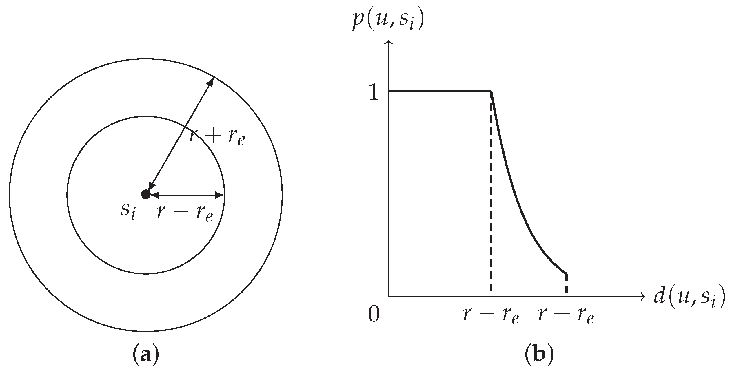
- The detection probability, of u by , used in this paper is (1).
4. Basics of the k-Layer Coverage
4.1. The Definition of k-Layer Coverage
4.2. “Zone 1 and Zone 1–2” Strategy
4.3. An Algorithm for Calculating the Radius of Zone 1
| Algorithm 1: |
| Input:, , and , where is the threshold, is the sensing range, and is the sensor-dependent parameter given in (1). Output: if ; or an -approximation of if .
|
- If , m, then for are 15.685m, 12.391m, and 8.749m, respectively.
- If , m, then for are 9.801m, 7.743m, and 5.468m, respectively.
5. Our k-Layer Coverage Scheme
5.1. The Case
- the first node in each even-numbered row (handled by line 6 of Algorithm 2),
- the last node in each row (handled by line 9 of Algorithm 2), and
- all nodes in row ℓ (handled by lines 11–18 of Algorithm 2).
| Algorithm 2: |
| Input: The derived by Algorithm 1, the length L of the ROI, and the height H of the ROI. Output: The designated locations of nodes.
|
5.2. The General Case
6. Experimental Results
7. Concluding Remarks
Author Contributions
Funding
Acknowledgments
Conflicts of Interest
Appendix A. Appendix: Balanced k-Layer Coverage

References
- Akyildiz, I.F.; Su, W.; Sankarasubramaniam, Y.; Cayichi, E. Wireless sensor network: A survey. Comput. Netw. 2002, 38, 393–422. [Google Scholar] [CrossRef]
- Huo, H.; Xu, Y.; Zhang, H.; Chuang, Y.H.; Wu, T.C. Wireless-sensor-networks-based healthcare system: A survey on the view of communication paradigms. Int. J. Ad Hoc Ubiquitous Comput. 2011, 8, 135–154. [Google Scholar] [CrossRef]
- Farsi, M.; Elhosseini, M.A.; Badawy, M.; Ali, H.A.; Eldin, H.Z. Deployment techniques in wireless sensor networks, coverage and connectivity: A survey. IEEE Access 2019, 7, 28940–28954. [Google Scholar] [CrossRef]
- Wang, B. Coverage problems in sensor networks: A survey. ACM Comput. Surv. 2011, 43, 32. [Google Scholar] [CrossRef]
- Mini, S.; Udgata, S.; Sabat, S. Sensor deployment and scheduling for target coverage problem in wireless sensor networks. IEEE Sens. J. 2014, 14, 636–644. [Google Scholar] [CrossRef]
- Rebai, M.; Snoussi, H.; Hnaien, F.; Khoukhi, L. Sensor deployment optimization methods to achieve both coverage and connectivity in wireless sensor networks. Comput. Oper. Res. 2015, 59, 11–21. [Google Scholar] [CrossRef]
- Wang, Y.C.; Tseng, Y.C. Distributed deployment scheme for mobile wireless sensor networks to ensure multilevel coverage. IEEE Trans. Parallel Distrib. Syst. 2008, 19, 1280–1294. [Google Scholar] [CrossRef]
- Dhillon, S.S.; Chakrabarty, K. Sensor placement for effective coverage and surveillance in distributed sensor networks. In Proceedings of the IEEE Wireless Communications and Networking Conference (WCNC’03), New Orleans, LA, USA, 16–20 March 2003; pp. 1609–1614. [Google Scholar]
- Yang, Q.; He, S.; Li, J.; Chen, J.; Sun, Y. Energy-efficient probabilistic area coverage in wireless sensor networks. IEEE Trans. Veh. Technol. 2015, 64, 367–377. [Google Scholar] [CrossRef]
- Yun, Z.; Bai, X.; Xuan, D.; Lai, T.H.; Jia, W. Optimal deployment patterns for full coverage and k-connectivity wireless sensor networks. IEEE/ACM Trans. Netw. 2010, 18, 934–947. [Google Scholar]
- Zou, Y.; Chakrabarty, K. Sensor deployment and target localization based on virtual forces. In Proceedings of the IEEE Infocom Conference (INFOCOM 2003), San Francisco, CA, USA, 30 March–3 April 2003; pp. 1293–1303. [Google Scholar]
- Wang, Y.; Wu, S.; Chen, Z.; Gao, X.; Chen, G. Coverage problem with uncertain properties in wireless sensor networks: A survey. Comput. Netw. 2017, 123, 200–232. [Google Scholar] [CrossRef]
- Nicules, D.; Nath, B. Ad-hoc positioning system (APS) using AoA. In Proceedings of the IEEE International Conference on Computer Communications (INFOCOM’03), Dallas, TX, USA, 30 March–3 April 2003; pp. 1734–1743. [Google Scholar]
- Klein, L.A. A Boolean algebra approach to multiple sensor voting fusion. IEEE Trans. Aerosp. Electron. Syst. 1993, 29, 317–327. [Google Scholar] [CrossRef]
- Sun, T.; Chen, L.J.; Han, C.C.; Gerla, M. Reliable sensor networks for planet exploration. In Proceedings of the IEEE International Conference on Networking, Sensing, and Control (ICNSC’05), Tucson, AZ, USA, 19–22 March 2005; pp. 816–821. [Google Scholar]
- Chakrabarty, K.; Iyengar, S.S.; Qi, H.; Cho, E. Grid coverage for surveillance and target location in distributed sensor networks. IEEE Trans. Comput. 2002, 51, 1448–1453. [Google Scholar] [CrossRef]
- Huang, C.F.; Tseng, Y.C. The coverage problem in a wireless sensor network. Mob. Netw. Appl. 2005, 10, 519–528. [Google Scholar] [CrossRef]
- Wang, H.L.; Chung, W.H. The generalized k-coverage under probabilistic sensing model in sensor networks. In Proceedings of the IEEE Wireless Communications and Networking Conference: Mobile and Wireless Networks (WCNC), Shanghai, China, 1–4 April 2012; pp. 1737–1742. [Google Scholar]
- Zhang, H.; Hou, J.C. Maintaining sensing coverage and connectivity in large sensor networks. Ad Hoc Sens. Wirel. Netw. 2005, 1, 89–124. [Google Scholar]
- Kershner, R. The number of circles covering a set. Am. J. Math. 1939, 61, 665–671. [Google Scholar] [CrossRef]
- Zou, Y.; Chakrabarty, K. Uncertainty-aware and coverage-oriented deployment for sensor networks. J. Parallel Distrib. Comput. 2004, 64, 788–798. [Google Scholar] [CrossRef]
- Zou, Y.; Chakrabarty, K. A distributed coverage- and connectivity-centric technique for selecting active nodes in wireless sensor networks. IEEE Trans. Comput. 2005, 54, 978–991. [Google Scholar] [CrossRef]
- Senouci, M.R.; Mellouk, A.; Oukhellou, L.; Aissani, A. Uncertainty-aware sensor network deployment. In Proceedings of the IEEE Globecom, Houston, TX, USA, 5–9 December 2011; pp. 1–5. [Google Scholar]
- Senouci, M.R.; Mellouk, A.; Oukhellou, L.; Aissani, A. An evidence-based sensor coverage model. IEEE Commun. Lett. 2012, 16, 1462–1465. [Google Scholar] [CrossRef]
- Senouci, M.R.; Mellouk, A.; Oukhellou, L.; Aissani, A. Efficient uncertainty-aware deployment algorithms for wireless sensor networks. In Proceedings of the IEEE Wireless Communications and Networking Conference: Mobile and Wireless Networks, Paris, France, 1–4 April 2012; pp. 2163–2167. [Google Scholar]
- Senouci, M.R.; Mellouk, A.; Oukhellou, L.; Aissani, A. WSNs deployment framework based on the theory of belief functions. Comput. Netw. 2015, 88, 12–26. [Google Scholar] [CrossRef]
- Ammari, H.M.; Das, S.K. Centralized and clustered k-coverage protocols for wireless sensor networks. IEEE Trans. Comput. 2012, 61, 118–133. [Google Scholar] [CrossRef]
- Elhoseny, M.; Tharwat, A.; Farouk, A.; Hassanien, A.E. K-coverage model based on genetic algorithm to extend WSN lifetime. IEEE Sens. Lett. 2017, 1, 7500404. [Google Scholar] [CrossRef]
- Liu, Q. K-coverage reliability evaluation for wireless sensor networks using 2 dimensional k / r×s / m×n:F system. In Proceedings of the 2018 12th International Conference on Reliability, Maintainability, and Safety (ICRMS), Shanghai, China, 17–29 October 2018; pp. 83–87. [Google Scholar]
- Özdağ, R. The solution of the k-coverage problem in wireless sensor networks. In Proceedings of the 2016 24th Signal Processing and Communication Application Conference (SIU), Zonguldak, Turkey, 16–19 May 2016; pp. 873–876. [Google Scholar]
- Rezaee, A.A.; Zahedi, M.-H.; Dehghan, Z. Coverage optimization in wireless sensor networks using gravitational search algorithm. J. Soft Comput. Inf. Technol. (JSCIT) 2019, 8, 20–31. [Google Scholar]
- Chen, Y.-N. Multilevel (k) Coverage Based on Probabilistic Sensing Model in Wireless Sensor Networks. Master’s Thesis, National Chiao Tung University, Hsinchu, Taiwan, June 2019. [Google Scholar]
- Chen, Y.-N.; Chen, C. Sensor deployment under probabilistic sensing model. In Proceedings of the 2nd High Performance Computing and Cluster Technologies Conference (HPCCT), Beijing, China, 22–24 June 2018; pp. 33–36. [Google Scholar]


| k | Case | Case | Case | Case |
|---|---|---|---|---|
| duplicate | duplicate | duplicate | duplicate and tri. pattern | |
| duplicate | duplicate | duplicate | duplicate and tri. pattern | |
| interpolation | interpolation | duplicate | duplicate and tri. pattern |
| k-Coverage by | Definition | det. prob. p Given by |
|---|---|---|
| k-expectation [18] | Equation (4) | |
| k-threshold [7] | Equation (1) | |
| k-layer (this paper) | see Definition 1 | Equation (1) |
| Size of the ROI | 1000 m × 1000 m |
| sensing range | 30 m |
| error tolerance used in Algorithm 1 | |
| sensor-dependent parameter used in (1) | either 0.05 or 0.08 |
| -Threshold [7] | Our -Layer | -Threshold [7] | Our -Layer | |||||
| # nodes | # nodes | # nodes | # nodes | |||||
| 0.7 | 7.133 | 7790 | 15.685 | 1672 | 4.458 | 19,781 | 9.803 | 4200 |
| 0.8 | 4.462 | 19,781 | 12.391 | 2640 | 2.789 | 50,369 | 7.744 | 6688 |
| 0.9 | 2.107 | 87,768 | 8.749 | 5226 | 1.317 | 223,520 | 5.468 | 13,161 |
| -Threshold [7] | Our -Layer | -Threshold [7] | Our -Layer | |||||
| # nodes | # nodes | # nodes | # nodes | |||||
| 0.7 | 2.377 | 206,424 | 15.685 | 5016 | 1.486 | 526,500 | 9.803 | 12,600 |
| 0.8 | 1.487 | 526,500 | 12.391 | 7920 | 0.929 | 1,343,811 | 7.744 | 20,064 |
| 0.9 | 0.702 | 2,350,872 | 8.749 | 15,678 | 0.439 | 6,005,520 | 5.468 | 39,483 |
| -Threshold [7] | Our -Layer | -Threshold [7] | Our -Layer | |||||
| # nodes | # nodes | # nodes | # nodes | |||||
| 0.7 | 1.426 | 952,070 | 15.685 | 8360 | 0.891 | 2,433,750 | 9.803 | 21,000 |
| 0.8 | 0.892 | 2,430,505 | 12.391 | 13,200 | 0.557 | 6,217,600 | 7.744 | 33,440 |
| 0.9 | 0.421 | 10,881,000 | 8.749 | 26,130 | 0.263 | 27,857,950 | 5.468 | 65,805 |
© 2020 by the authors. Licensee MDPI, Basel, Switzerland. This article is an open access article distributed under the terms and conditions of the Creative Commons Attribution (CC BY) license (http://creativecommons.org/licenses/by/4.0/).
Share and Cite
Chen, Y.-N.; Lin, W.-H.; Chen, C. An Effective Sensor Deployment Scheme that Ensures Multilevel Coverage of Wireless Sensor Networks with Uncertain Properties. Sensors 2020, 20, 1831. https://doi.org/10.3390/s20071831
Chen Y-N, Lin W-H, Chen C. An Effective Sensor Deployment Scheme that Ensures Multilevel Coverage of Wireless Sensor Networks with Uncertain Properties. Sensors. 2020; 20(7):1831. https://doi.org/10.3390/s20071831
Chicago/Turabian StyleChen, Yu-Ning, Wu-Hsiung Lin, and Chiuyuan Chen. 2020. "An Effective Sensor Deployment Scheme that Ensures Multilevel Coverage of Wireless Sensor Networks with Uncertain Properties" Sensors 20, no. 7: 1831. https://doi.org/10.3390/s20071831
APA StyleChen, Y.-N., Lin, W.-H., & Chen, C. (2020). An Effective Sensor Deployment Scheme that Ensures Multilevel Coverage of Wireless Sensor Networks with Uncertain Properties. Sensors, 20(7), 1831. https://doi.org/10.3390/s20071831