The consideration of taking random samples of sensor locations provides additional degree of freedom for controlling the sidelobes. To achieve the desired mainlobe accompanied by reduction of the sidelobes, it is required to select a subset of connected and collaborative sensors from candidate sensors within the same coverage area of each th source–destination pair.
This sampling is assumed to be as Latin distributed random variable which represents the whole coverage area considering the fluctuations/shadowing effects in the channel. It depends on the distance among the selected collaborative sensors, whereas the sensors are close to each other, while the base station is located far from these selected collaborative sensors. Moreover, the network can be viewed as homogeneous and the power attenuation due to different paths are unequal. Therefore, we can either adjust the gains of the receivers or the power/the number of the collaborative sensors participating in CB by adjusting the weights.
6.1. The Sensor Selection Algorithm
Node selection procedure works on the basis that the positions of the sensors forming an antenna array are selected such that their mutual phase offset due to their locations creates a coherently combined signal at the cluster head. Consequently, the node selection algorithm involves carefully selecting the best position for each collaborative sensor and then positioning according to the logical connectivity such that the beampattern is optimal. Assume be a set of collaborative sensors to be selected from , i.e., , to form beampattern towards the base station. The path connectivity assigns a set of collaborative sensors to each source–destination pair that forms a specific topology. Each cluster consists of many sensors, thus the mainlobe of the beampattern is unstable for different number of of different subsets . This occurs as long as the coverage area does dynamically change according to IoT environment as well as the requirements of the applications in that environment. It is necessary to take into consideration these two conditions to maximize mainlobe towards the intended base station and minimize the sidelobes.
We have developed an algorithm for sensor selection based on robust optimization scheme satisfying certain objective functions. First, to find an optimal solution for uncertain objective function which guarantees that the sidelobe levels at the direction of intended base station are below a certain prescribed value. Second, to find an optimal solution that is stable under fluctuations of the channel environments.
However, it seems a challenge to find a robust optimal solution for the objective function on a continuous optimization problem with uncertainty fluctuations in the collaborative sensors. This is because of the difficulty of realizing the gain achieved from the fluctuations in input variables to get an optimal solution. Hence, to assess the robustness of a solution for the objective function, there are common measures to calculate the expected fitness function taking into account the input variable fluctuations and their probability of deployment via a probability distribution function over the whole input variable space , where is the problem’s dimension.
As mentioned in the previous section, the spacing among the collaborative sensors affects the beampattern shape of the antenna array. Thus, selecting random sensors positions i.e., uncertain sensor positions may lead to positions errors. However, the minimum SLL of an antenna array with fixed and selected sensors positions is higher than that of the antenna array with randomly selected sensors if the number of antenna array is the same, since the distance among the randomly selected sensors has maximum Euclidean distance corresponding to a certain hop-distance which is considered to be a practical metric for modeling spatially random sensor network. Specifically, the connectivity in terms of estimating the area of interest is defined by maximum distance that can be covered in multihop paths. Furthermore, the maximum Euclidean distance is directly related to the estimated hop-distance which is equal to the least number of hops overall multihop paths between any two locations. Therefore, CPSO is used for the optimization of sensor selection whereas the topology of random selection becomes regular topology such as linear, mesh, tree, or ring and the SLL deteriorates further. The objective function is given as
The calculation of the objective function takes into consideration the number of distributed collaborative sensors sampled and the possibility of connectivity via a probability distribution function of deployment over the coverage area , where is the problem’s dimension. The required number and topology of distributed sensors N must first be decided to construct the antenna elements ℵ in the network.
Consider
N as the total number of sensors, the number of collaborative sensors to be selected is
, where
, and the number of distributed collaborative sensors sample of one active cluster to be tested in each iteration be
. The number of distributed collaborative sensors samples for achieving an optimal solution is an important factor, since each selected sensor must share the transmission range among others within the active cluster. This implies that the characteristic parameters of a CB of the selected sensors must maintain their stable values as the number of samples increases. Moreover, while testing one group or a group of sensors, we need to check if beamforming of the corresponding distributed collaborative sensors sample increases the mainlobe and decreases sidelobes in the intended and unintended direction(s), respectively. Thus, the minimum number of these samples can be determined when the mainlobe and sidelobes reach their stable values. To avoid occurrence of grating lobes, the interspace among sensors should satisfy
[
20]. The selection process can be summarized as follows:
- Step 1
Each sensor starts to explore the neighbors in all directions using randomly directed antenna scheme. Assuming that sensors in the cluster know their distance relative to the cluster head by directly communicating with the base station, then the weights of the signal transmitted and received by the cluster head can be computed.
- Step 2
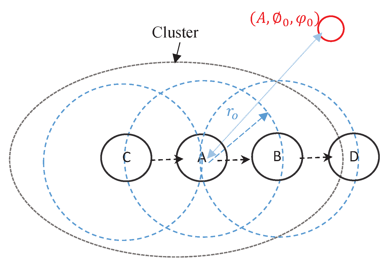
Suppose that the cluster head and its neighbors are arranged in a specific network topology such as linear, mesh, or random. Then, the cluster head is at approximately equal distances from each other in linear and mesh topology, meanwhile it is not equal in random topology. Hence, assume that
acts as the reference of the active cluster to select the collaborative sensors to perform the CB. We need to check the closest selected collaborative sensors
within transmission range of cluster head as
- Step 3
Sensors are selected to form an antenna array that adjusts its own radiation pattern to radiate the beampattern in certain direction and reject the signals from other directions. This is controlled by the weighted signal of the collaborative sensors which are computed and the signal is transmitted to the cluster head based on robust particle swarm as discussed in
Section 6.2 to satisfy the objective function defined in Equation (
20). The memetic objective function shows that these weights could be adapted to change based on the signal environment in terms of fluctuations/shadowing in the channel. Therefore, the optimal radiation pattern can be obtained through maximizing the mainlobe and minimizing the sidelobes by perturbing the positions of selected collaborative sensors in the antenna array.
6.2. The Robust Canonical Particle Swarm
PSO is an iterative, population-based intelligent computational algorithm which searches for optimal solution for non-linear continuous problems. The performance of PSO depends on the power of the solutions’ population that endorse it to find several optimal solutions, i.e., particles over multiple generations. Therefore, one improvement would be to generate randomizing potential particles and continue using the dynamic distances among the particles to dictate communications with selected particles. However, such as technique requires intensive computations to determine these distances, and therefore, PSO is not viable for larger dimensions for the following reasons.
PSO can struggle as it can be difficult for the combination of the number of particles, i.e., swarm to enlarge the search space size to converge on an optimal solution, often getting stuck in local optimal.
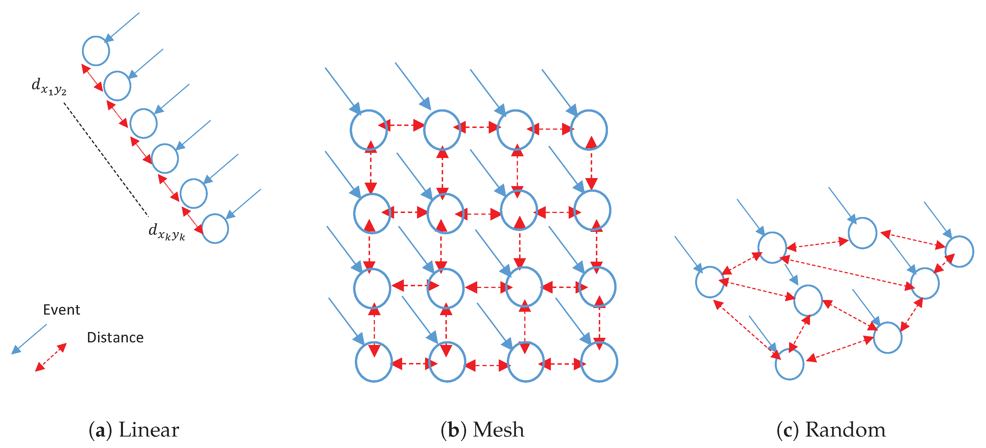
The particles are connected as a topology which enables several communication paths among its members and the way the swarm is searching the landscape. Since the neighborhood topology changes the pattern of the swarm, convergence and diversity differ from one topology to another. In ring topology known as local PSO the information is slowly distributed among the particles. Therefore, using the ring topology slows the convergence rate because the optimal solution must propagate through a few neighborhoods before affecting all particles in the swarm. Meanwhile, mesh topology uses a kind of fully connected topology that is known as global PSO . The communication among the particles is expedition, and swarm quickly moves towards the best solution. Because of the cost of neglecting part of the search space, the population may fail to explore outside of local regions causing the swarm to be trapped in local optimal solution.
PSO suffers from the dual problems of outdated memory due to the environment dynamism and diversity loss, due to convergence.
PSO does not always work perfect and may need tuning of its behavioral control parameters such as weight inertia and constriction factor.
The following points clarify the differences between PSO and CPSO:
Particles in CPSO possess memory of the best location visited in and its fitness value.
Every particle shares information with every other particle in the swarm and there is a single attractor representing the best location of the entire swarm.
CPSO provide more control to parameters of the swarm behavior by mathematical operators such as ⊗, ⊕, and ⊙ for increasing and decreasing the inertial weight and velocity clamping.
The PSO algorithm starts as follows: an initial swarm of particles as one-dimensional vector
are generated at random. These particles communicate and move in the research space to allocate optimal solution and reach at optimal area. The position of particles is changed by adding a velocity to the current position:
. In comparing PSO with CPSO, the proposed optimization algorithm exists as a swarm of particles, i.e., sensors and each particle
ı resides at position
. These particles move with a certain velocity
over the search space. Each position is associated with a fitness value given by the objective function during several iterations of evaluations
. For
N-dimensional problem, the position and velocity can be specified by
matrices as follows
As mentioned,
ℵ defines the number of particles/sensors in the swarm. Each row of the position matrix represents a possible solution to the optimization problem after evaluating the objective function
multiplied by connectivity indicator factor
defined as follow
Hence, the best position is defined as the local or personal-best
achieved by the evaluation of the objective function for collaborative sensors during the first iteration of selection as follows.
Moreover, each particle knows its
best value so far, which corresponds to experience of each particle. Among all iteration of all collaborative clusters, a new position is considered to be a global-best position
and is defined by
Moreover, each particle may either achieves a better position or does not by adjusting its velocity based on the evaluation of the objective function defined in Equation (
20) in the previous position as well as the best previous positions of all particles. Specifically, each particle tries to adjust the velocity based on the following information to modify its position and refine its own weight:
After a certain number of iterations,
all particles of the swarm converge towards positions that are optimal either locally or globally. The degree of influence among the personal and global-best solutions should be defined by coefficients. For instance, the personal position is defined by coefficient
, meanwhile the influence of the best global or neighborhood exchange solution is defined by a coefficient
. Accordingly, updating the velocity and position of an
th particle at
th iteration is defined mathematically as
The position of the
th particle/sensor for the next iteration is updated such that
, where
is the cognitive parameter,
is the social parameter,
is defined as the inertia weight index that tries to explore a new cluster, and
is a random number within [0,1]. The ratio of
determines the importance of
and to
. There are many mays to implement the constriction coefficient
. One of the simplest methods is shown in Equation (27), whereas the first term of expresses the previous velocity of the information vector (in other word the personal-best vector before starting to change particles/sensors information with their neighbors). Meanwhile, the second and third terms are used to change or update the velocity of the information vector from personal-best vector to global-best. Without the second and third terms, the vector will keep on moving in the same direction until it hits the boundary. The inertia weight
, regulates the influence of the previous velocity
on the new velocity
, and it should not be confused with beamforming coefficient weights, whereas the inertia weight is a constriction coefficient, which helps to balance global exploration and local exploitation, and thus helps in preventing velocity explosions. It is defined as follows [
41]:
The Clerc’s constriction method is used [
45], where
is commonly set to 4.1 which helps to control the convergence of particles, whereas
, and
is set as a constant value. Therefore, the constricted particles converge without using any velocities values at all, i.e., removal of velocity clamping facilitates larger exploration abilities of the swarm. This implies a swarm behavior that is eventually limited to a small area of the feasible search space containing the optimal solution. However, Equations (27) and (
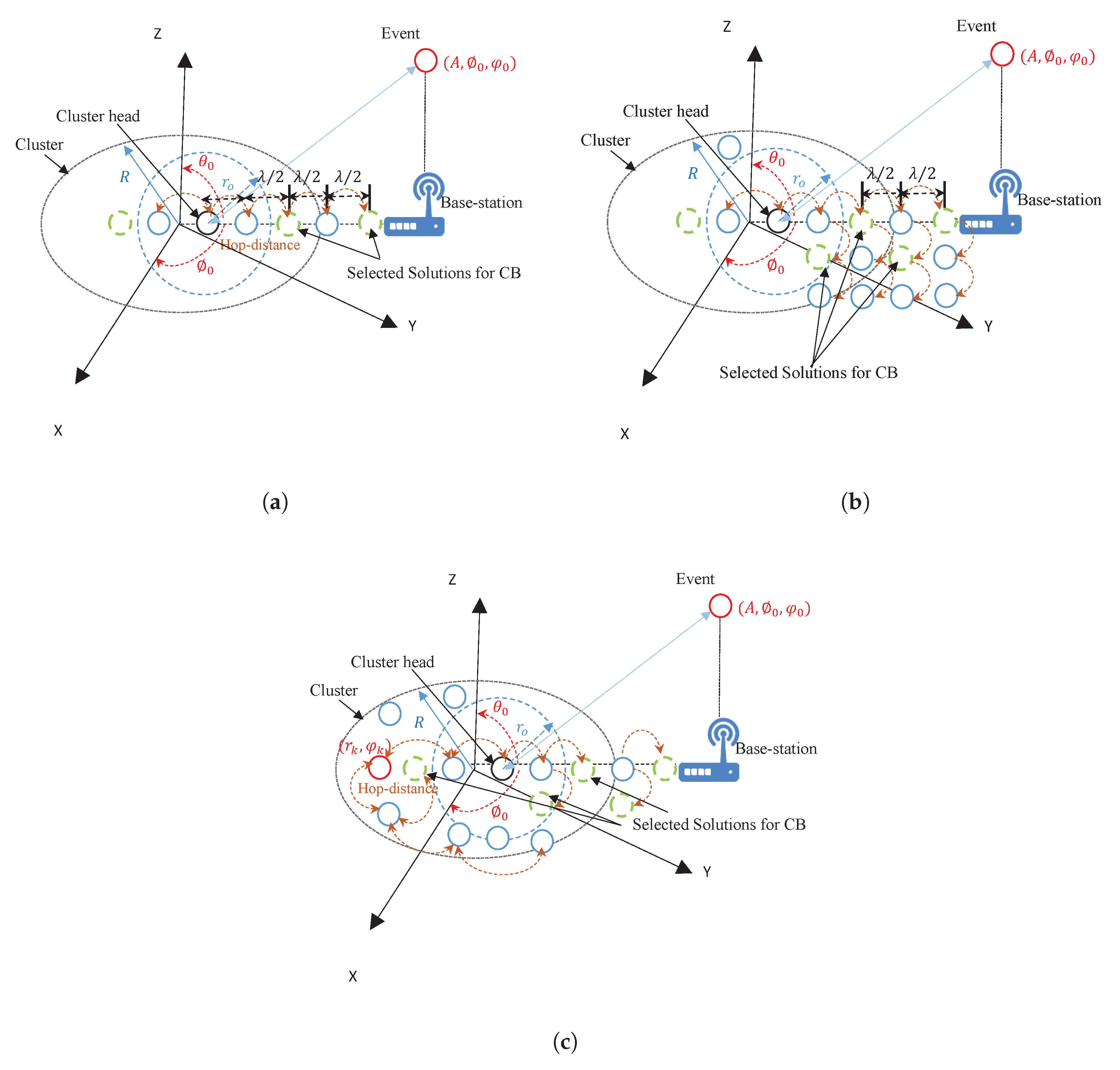
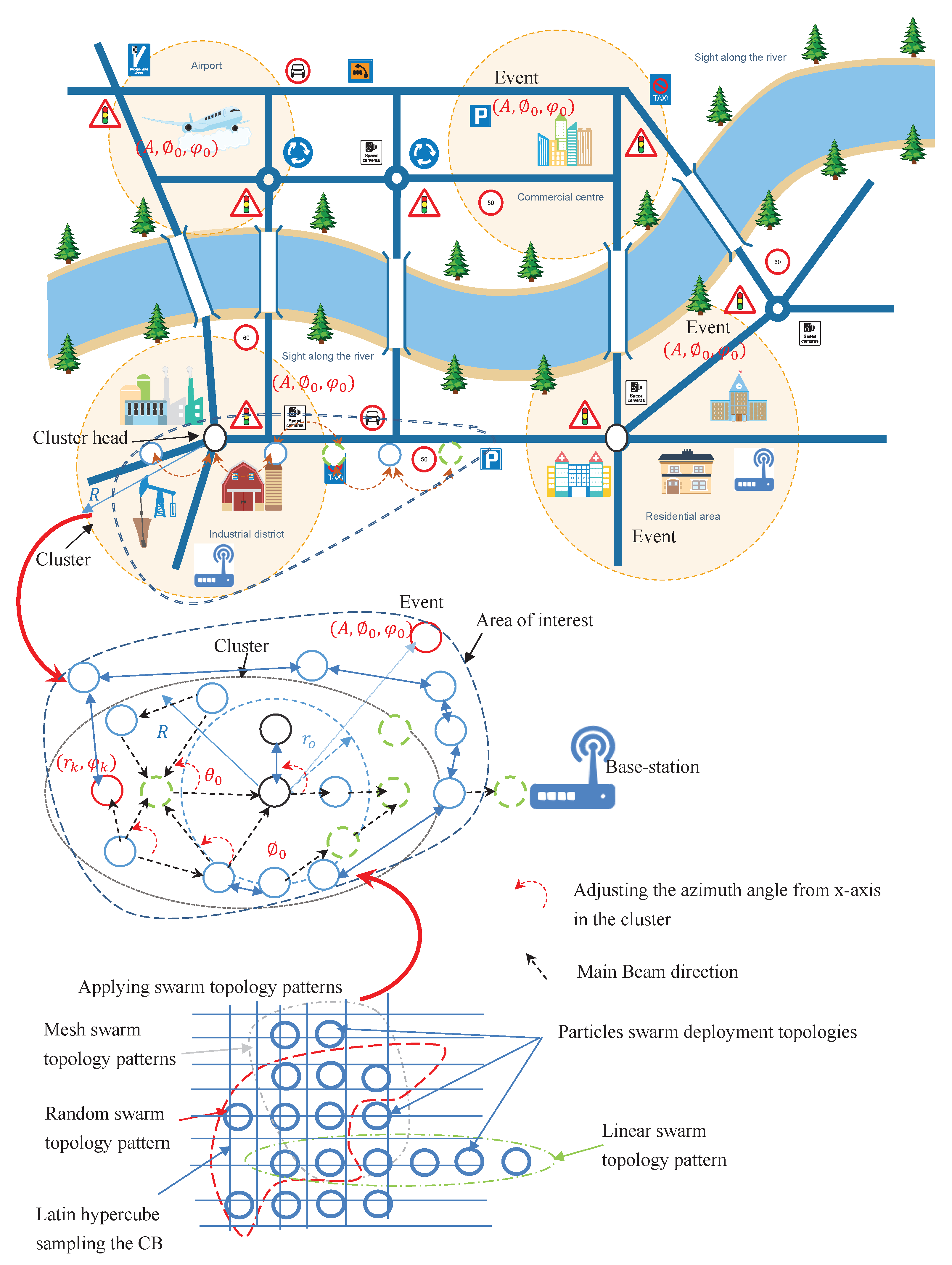
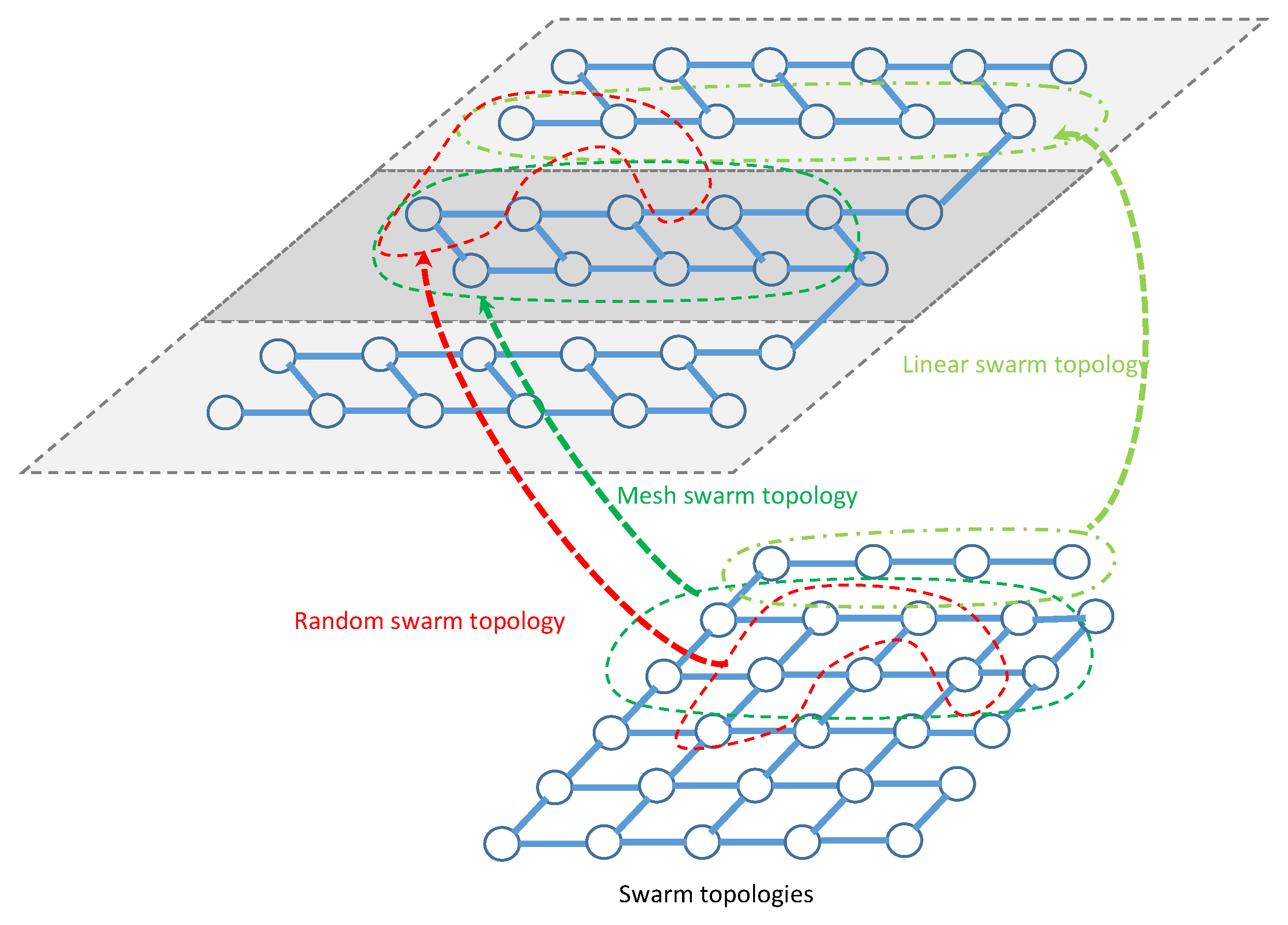
28) are formulated such that the CPSO has no problem-specific parameters addressing all efficiency of exhaustive search over all possible solutions. Indeed, a logical connectivity describes how directional beamforming affects a network topology and how the information is shared and transmitted by one sensor to another. These topologies are created by orientating the mainlobe direction of the selected collaborative sensors based on sharing and exchange information of the locations from their neighborhood towards the geometric center of the cluster. Hence, these topologies may have prefect and imperfect information of the position of other sensors. According to Equation (
21), the topology of the selected collaborative sensors as shown in
Figure 5 will enable the CPSO to have a higher diversity and then being able to find global optimal solution better than all topologies as shown in
Figure 6 which are well suited for finding local optimal solution. After a certain number of iterations
, a custom topology creates group of collaborative sensors with a maximum mainlobe and minimum sidelobe by maximum of
out of
ℵ sensors or particles in total. It should be noted that the purpose of using the present swarm topology is to combine the benefits of all type of topologies in terms of linear, mesh, and tree. We rewrite the objective function as
subject to
The objective function in Equation (
29) can be applied to both isotropic and realistic antenna patterns according to the type of IoT applications as well as their requirements. However, there is no closed-form expression of Equation (
29) for realistic antenna model or even for a simplified antenna model. Furthermore, it is not possible to obtain closed-form expression for the optimization problem hence an approximate solution is needed.
We adopt a popular approach for this approximation by means of Latin distribution of collaborative sensors sampled for the fitness value of the objective function in an area of interest [
44]. For the approximation of the maximum/minimum values of the objective function, this means that
n samples must be taken out of an area of interest
and the
of the sampled fitness value would be returned as


