Counter a Drone in a Complex Neighborhood Area by Deep Reinforcement Learning


Abstract
1. Introduction
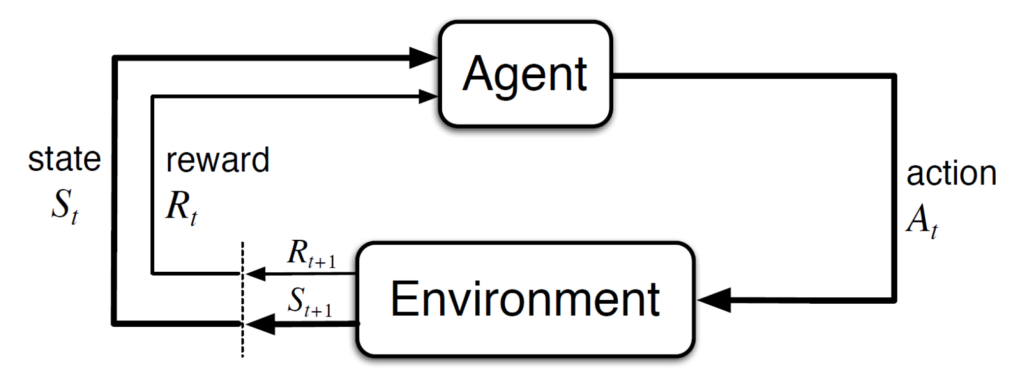
2. Methods
3. DRL Model Definition
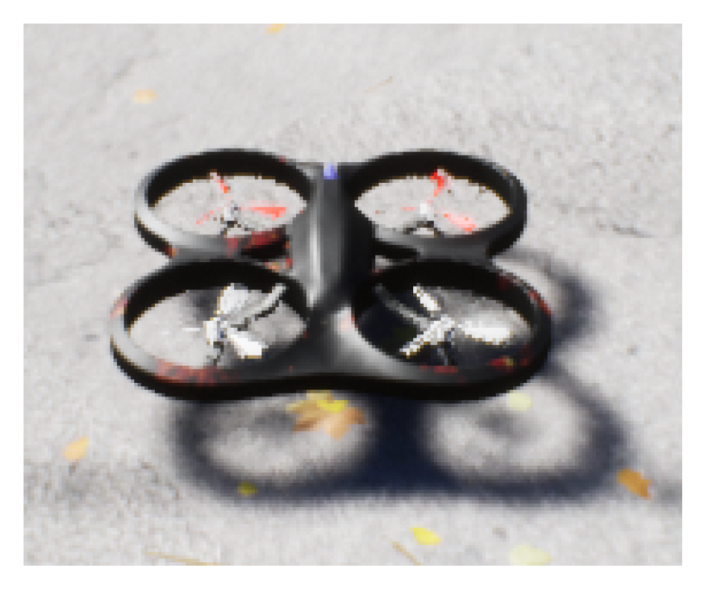
3.1. Tools
3.2. Model
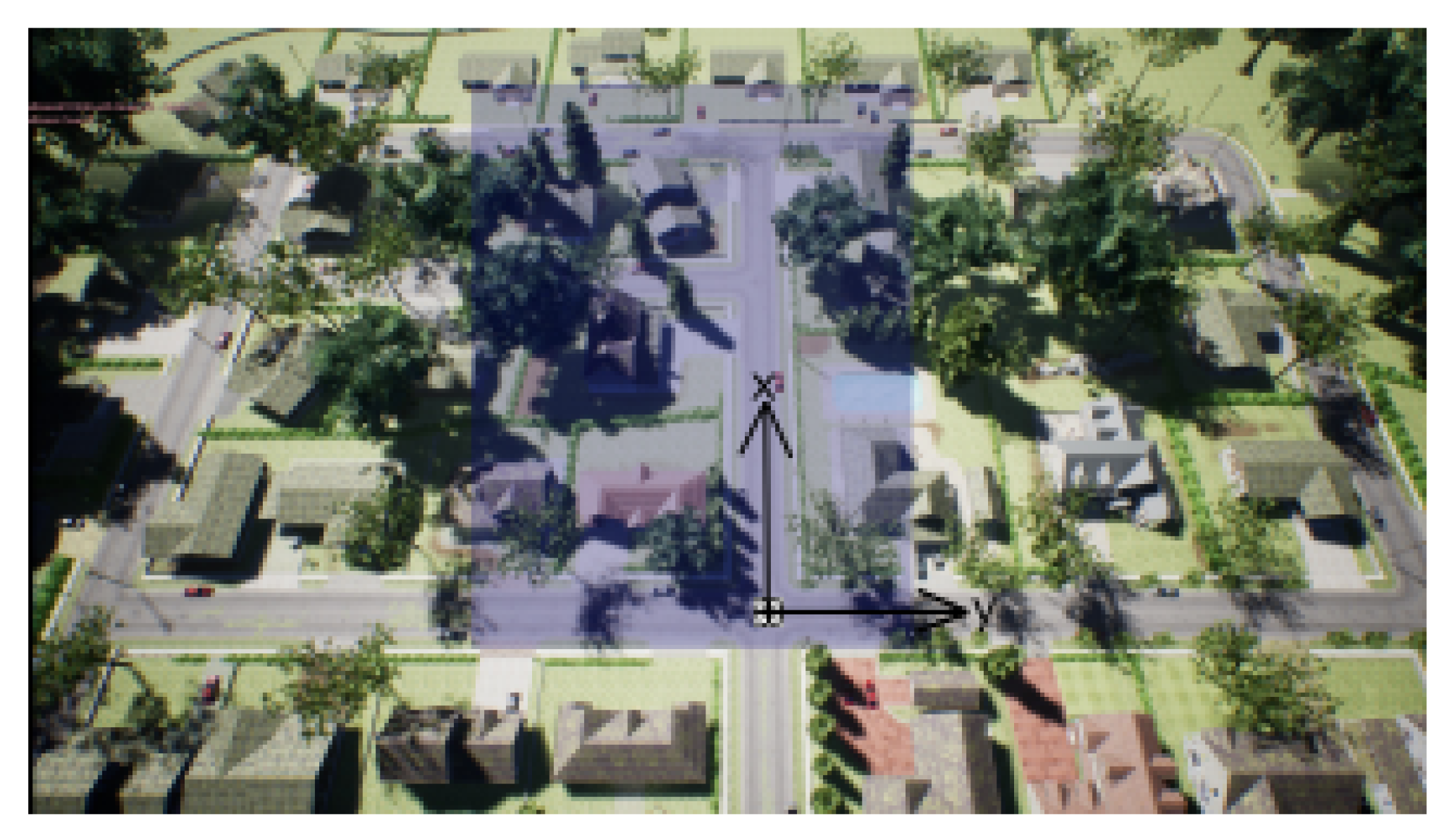
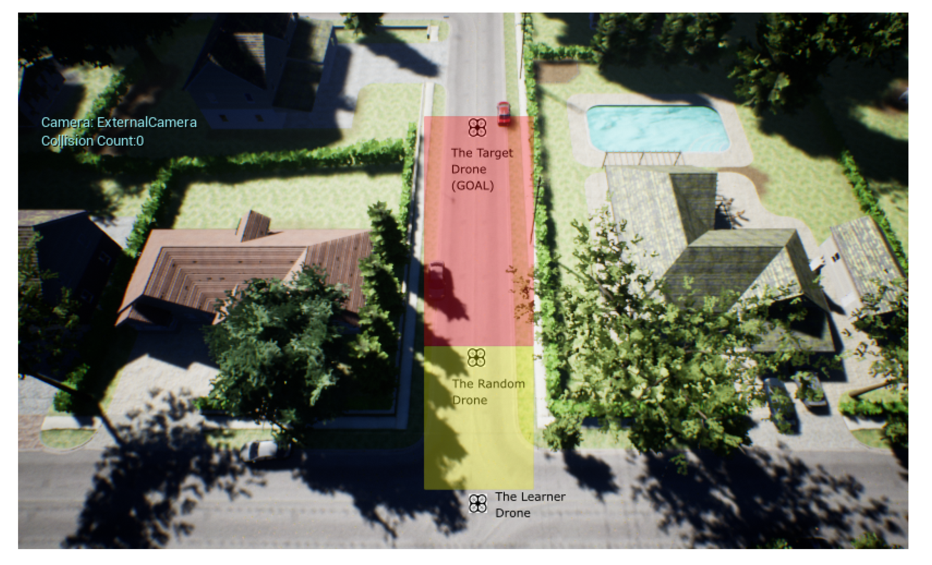
3.2.1. Environment
3.2.2. State Representation
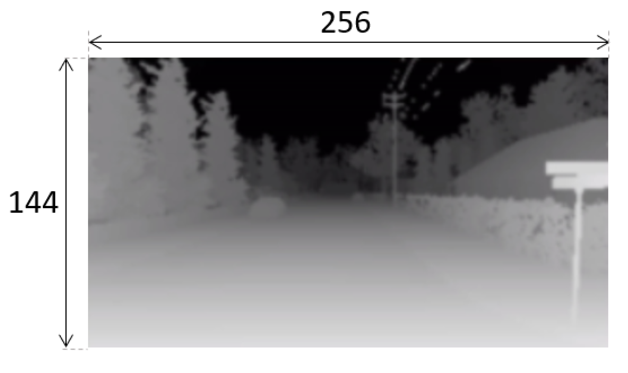
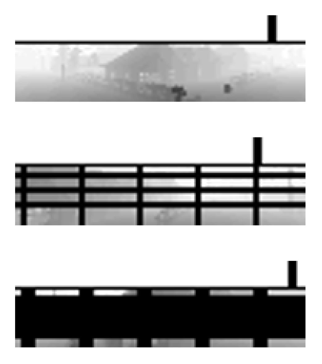
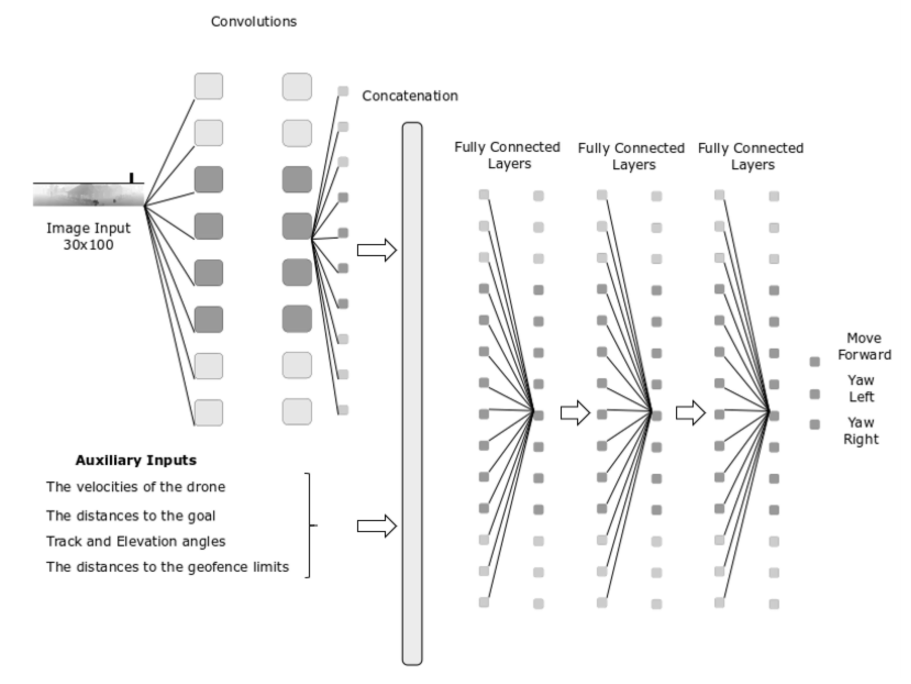
- Image
- Auxiliary Inputs
- The velocity of the agent in x and y directions:
- The distance from the agent to the goal in x and y directions and the Euclidean distance:
- Track and the elevation angles between the agent and the goal:
- The distances to the four geofence limits
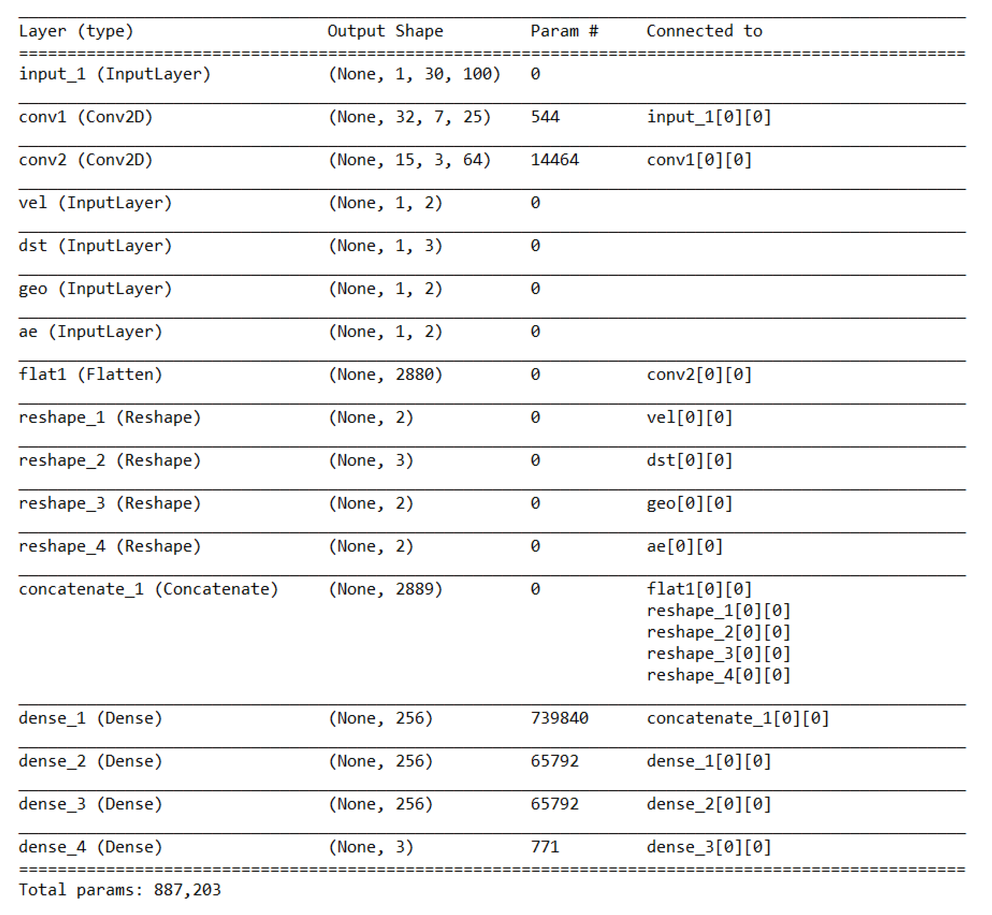
3.2.3. Agent’s Neural Network
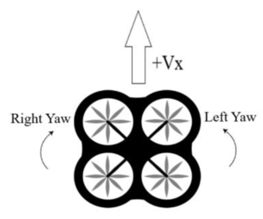
3.2.4. Actions
- Straight: Straight movement in direction of the heading with speed equal to 4 m/s
- Yaw left: Rotate clockwise around z axis with a 30 deg/s angular speed
- Yaw right: Rotate counter-clockwise around z axis with a 30 deg/s angular speed
3.2.5. Rewards
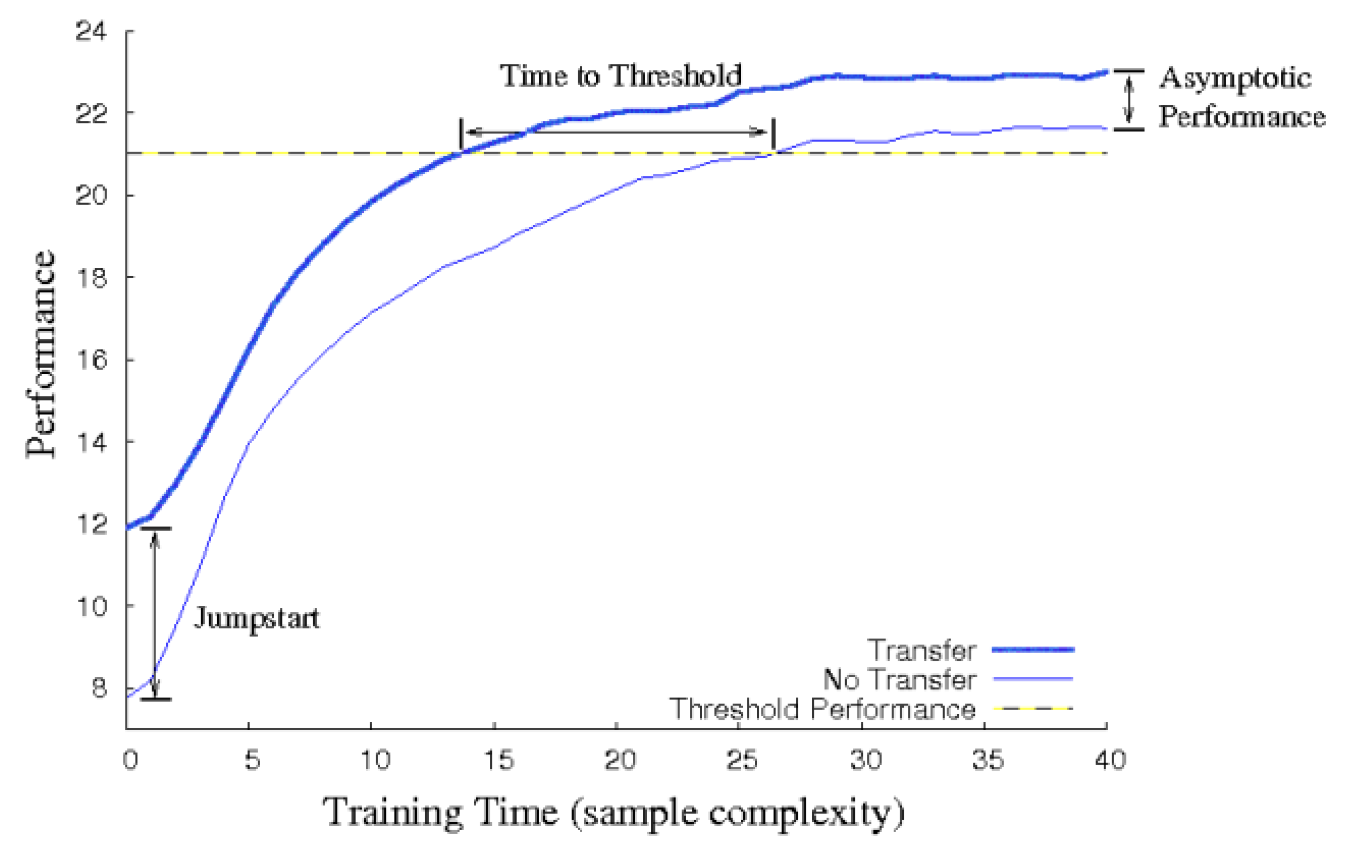
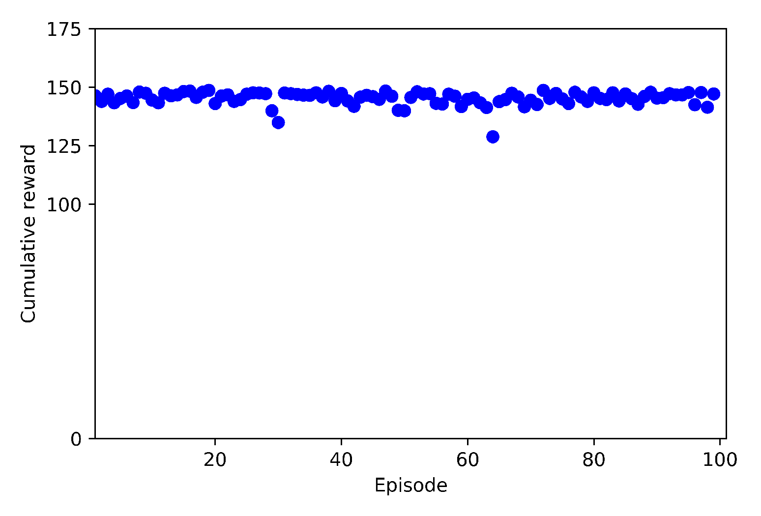
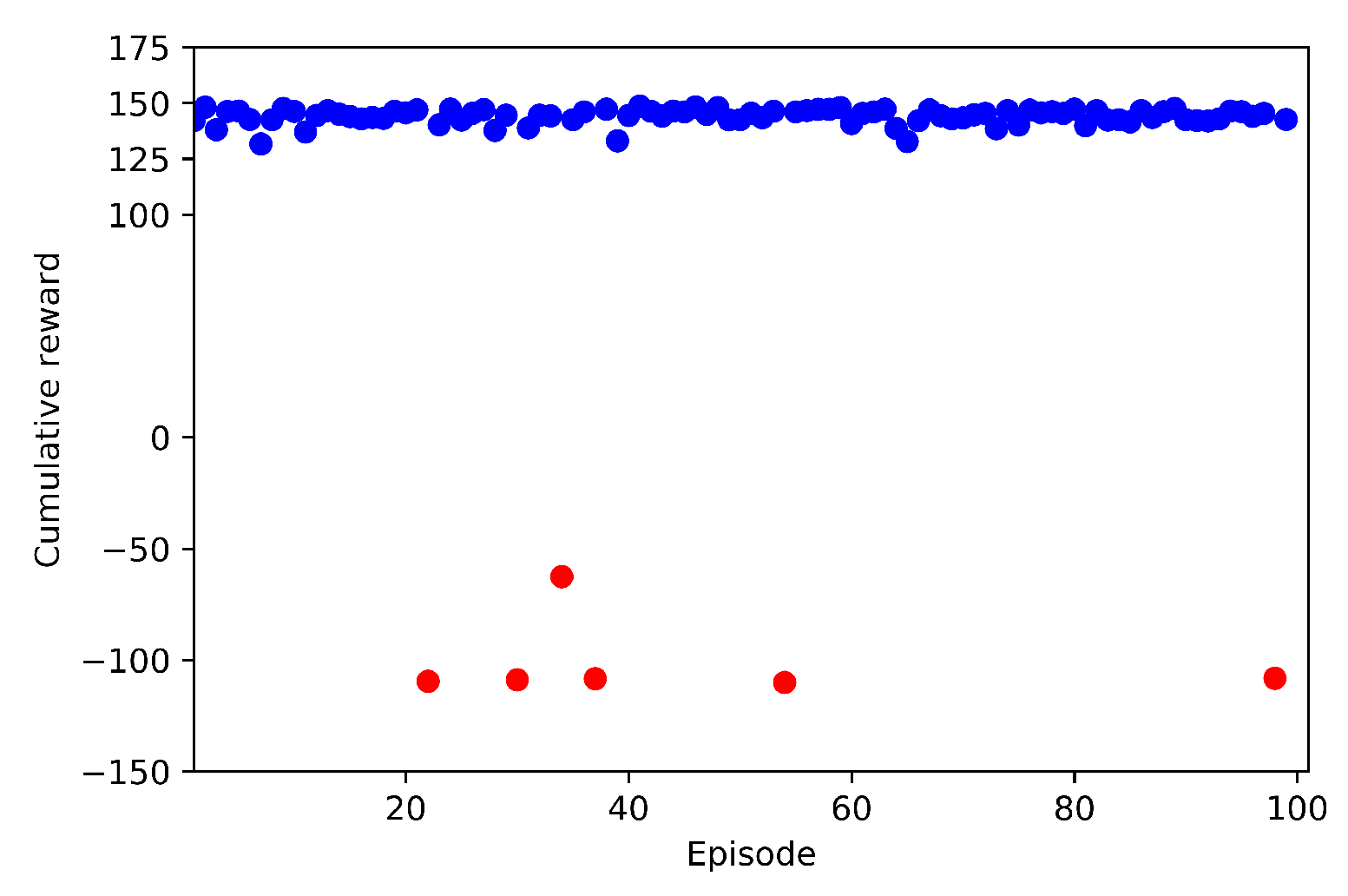
4. Training Analysis & Results
4.1. Training Setup
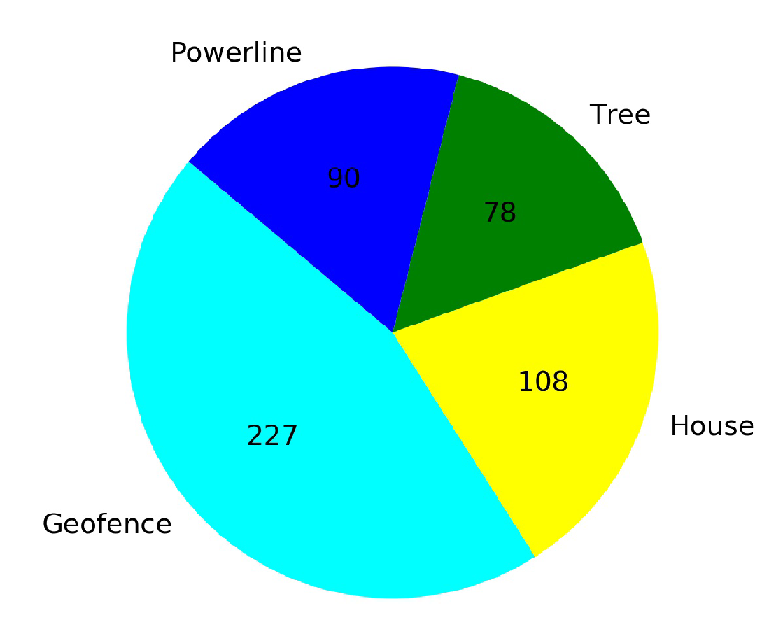
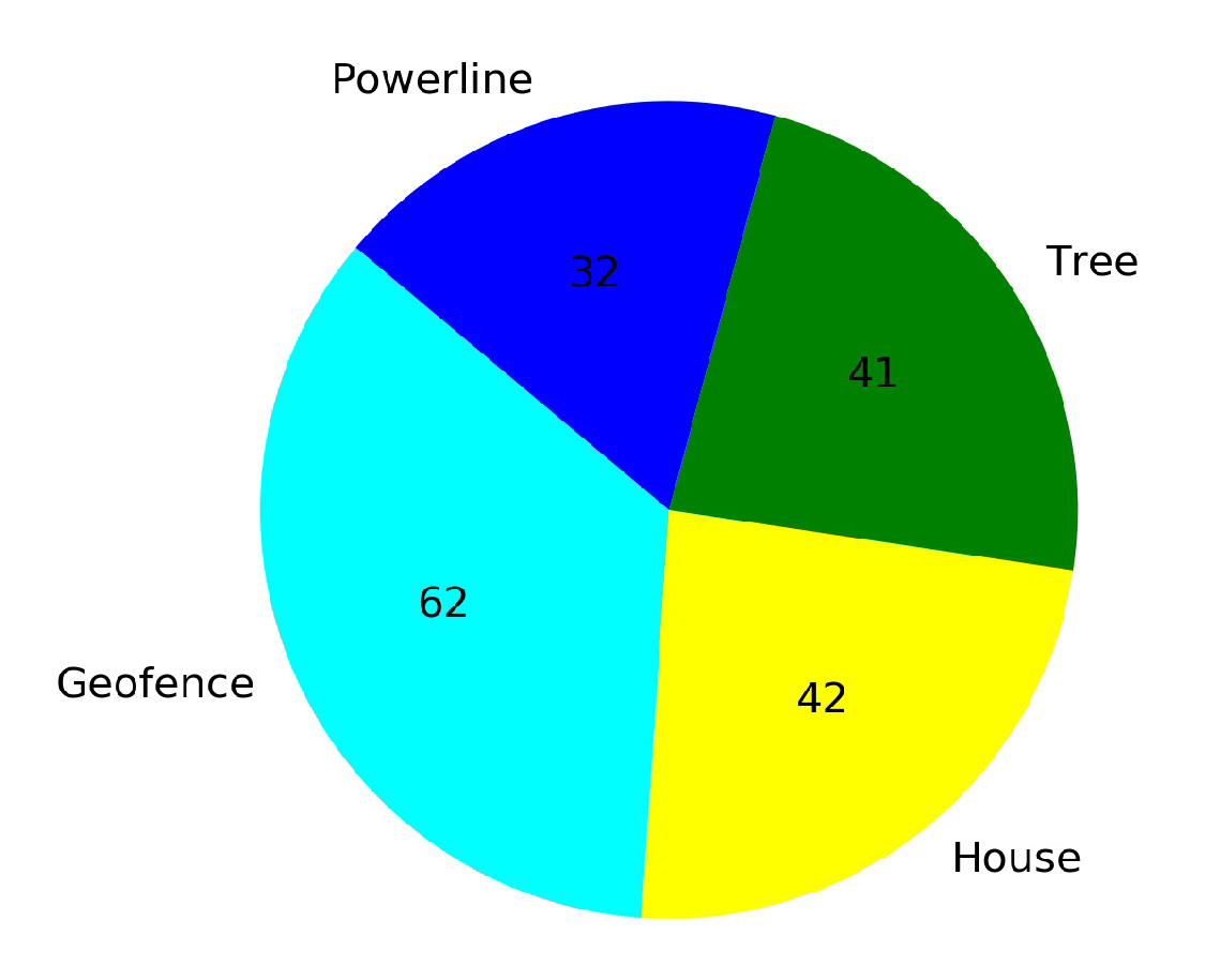
4.2. Definition of Cases
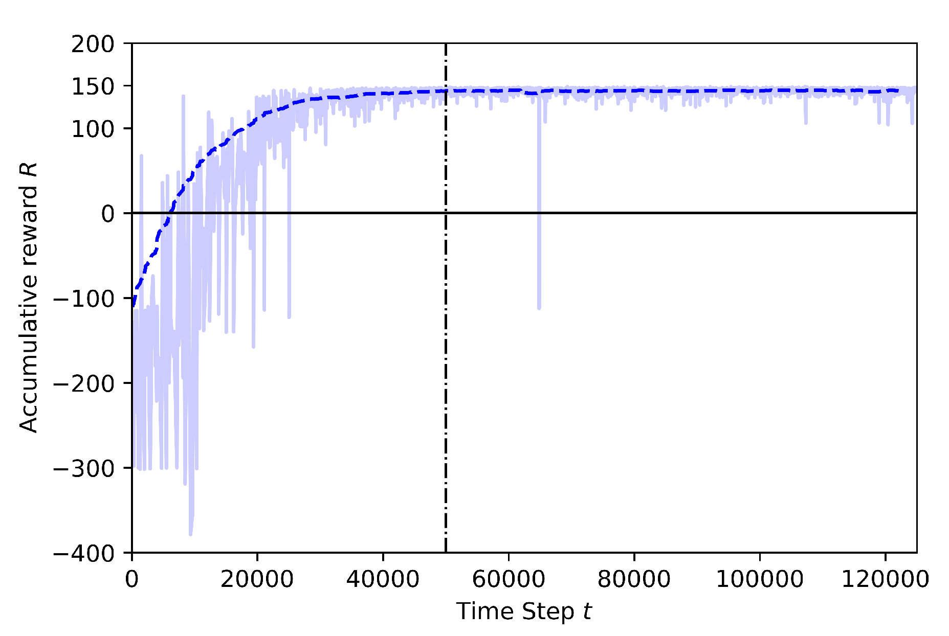
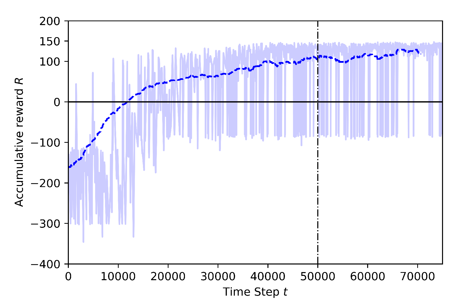
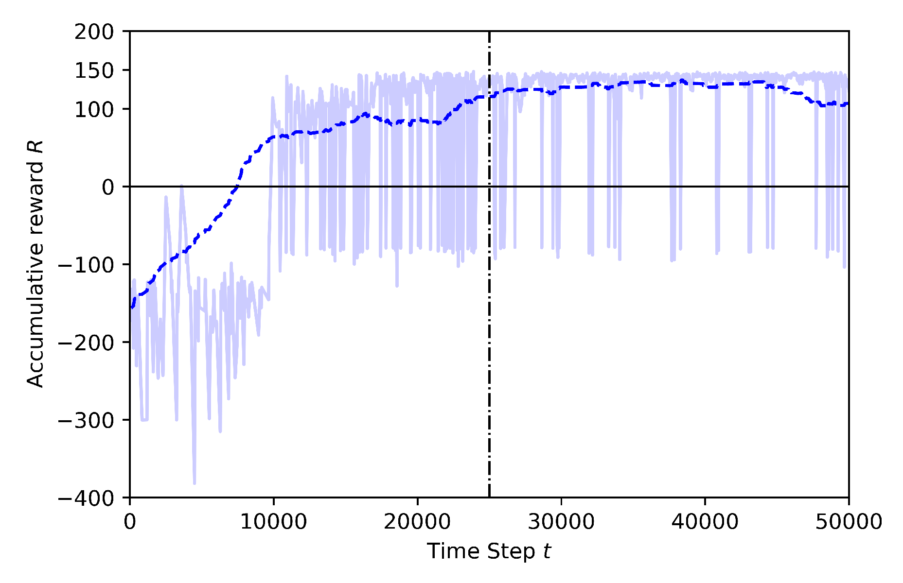
4.3. Training Results
4.3.1. Case 1: Training at 30 m Height
- Baseline: Training including geofence and target drone
- Case 1.1: adding a stationary third drone
- Case 1.2: adding a stationary third drone and using pre-trained model from Baseline
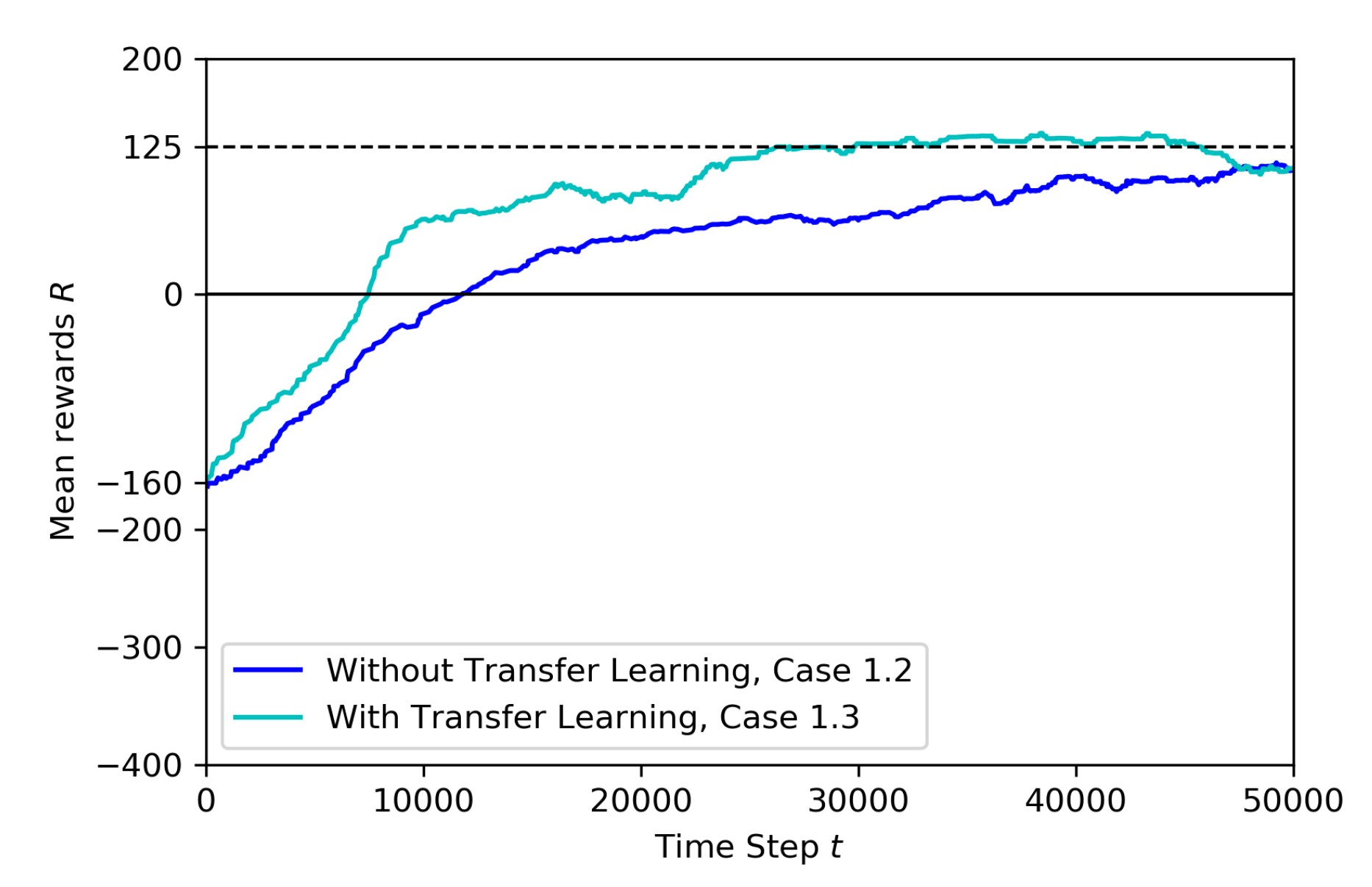
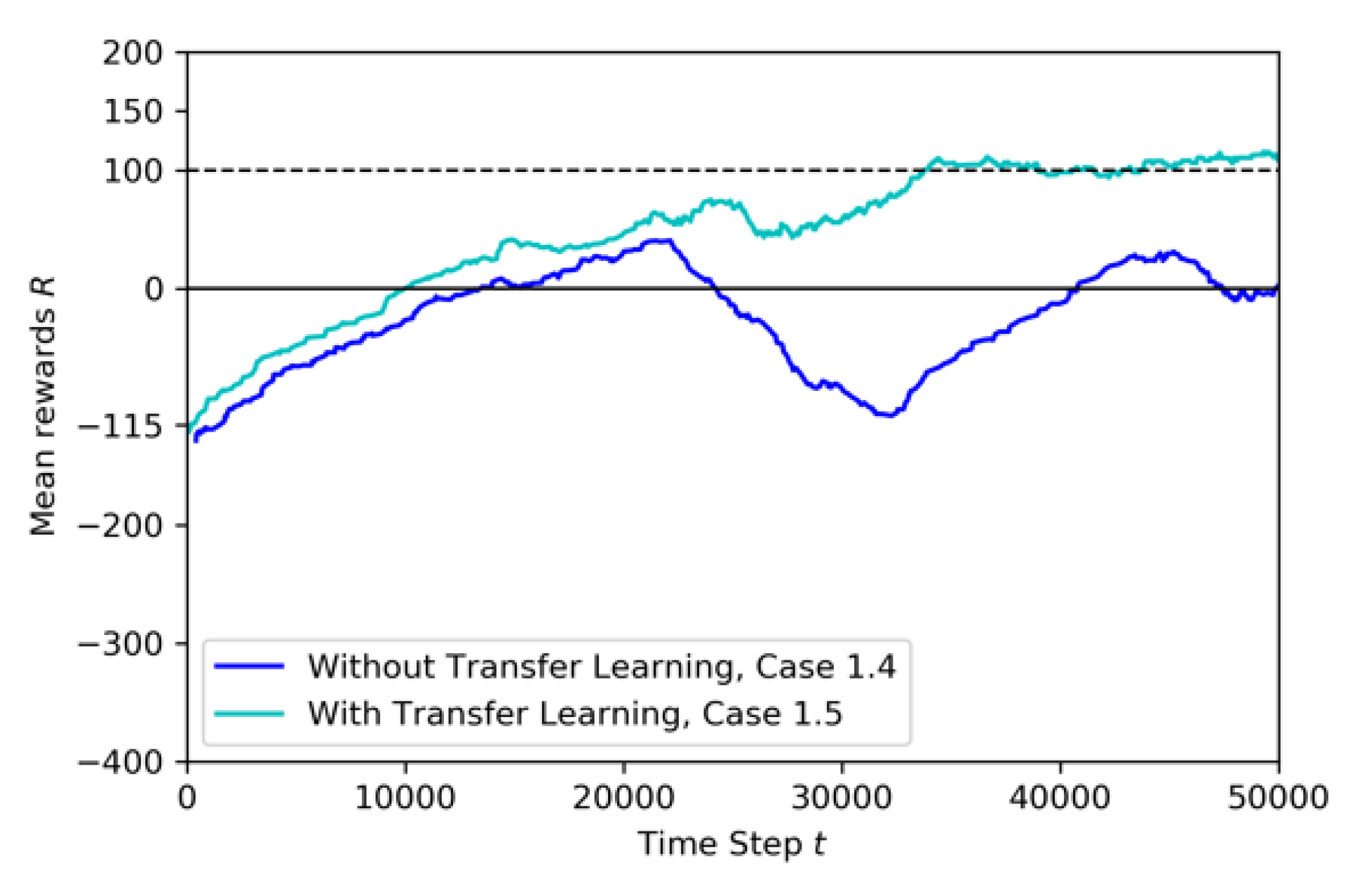
- Case 1.3: adding movement to the third drone
- Case 1.4: adding movement to the third drone and using pre-trained model from Baseline
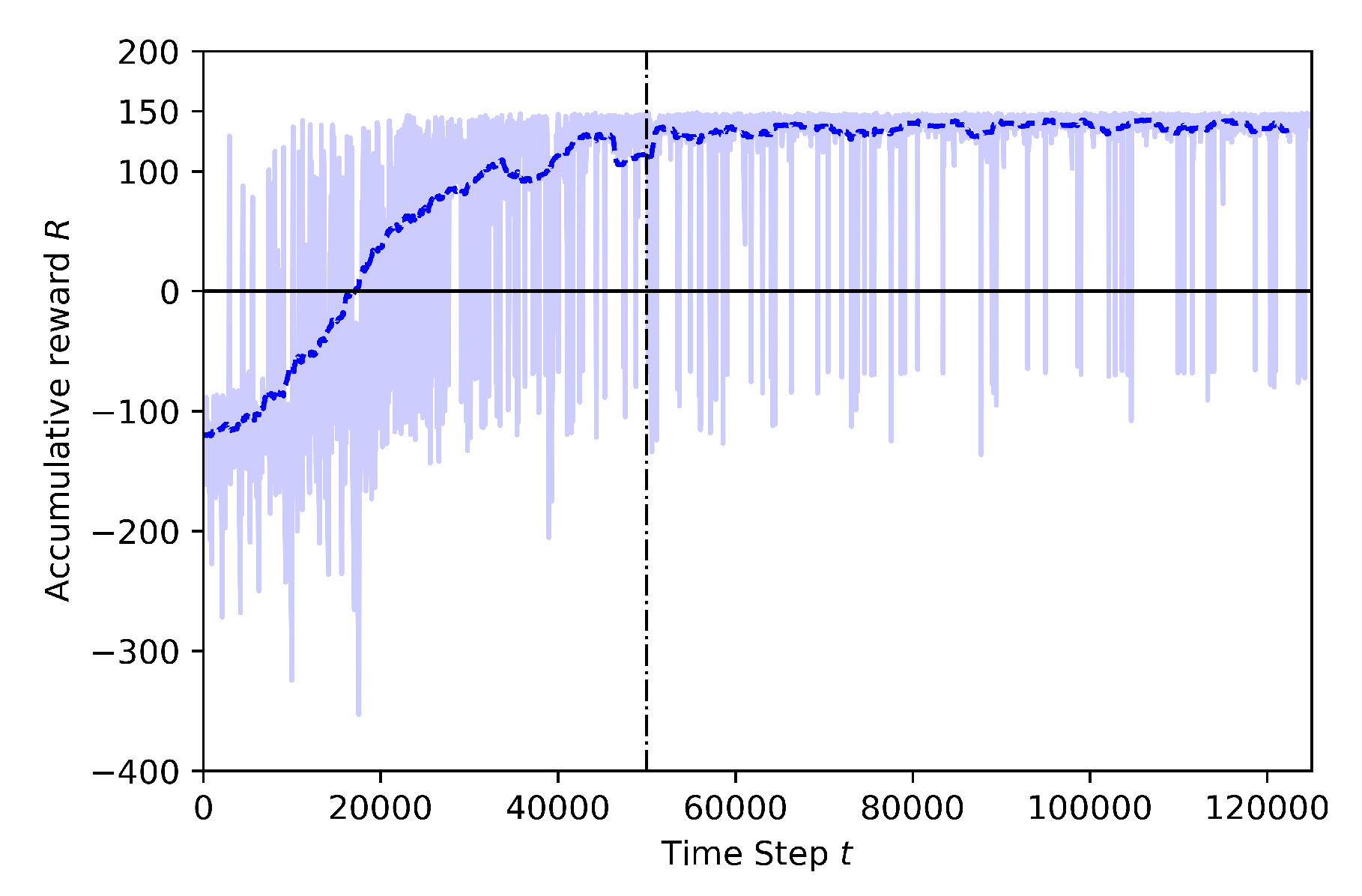
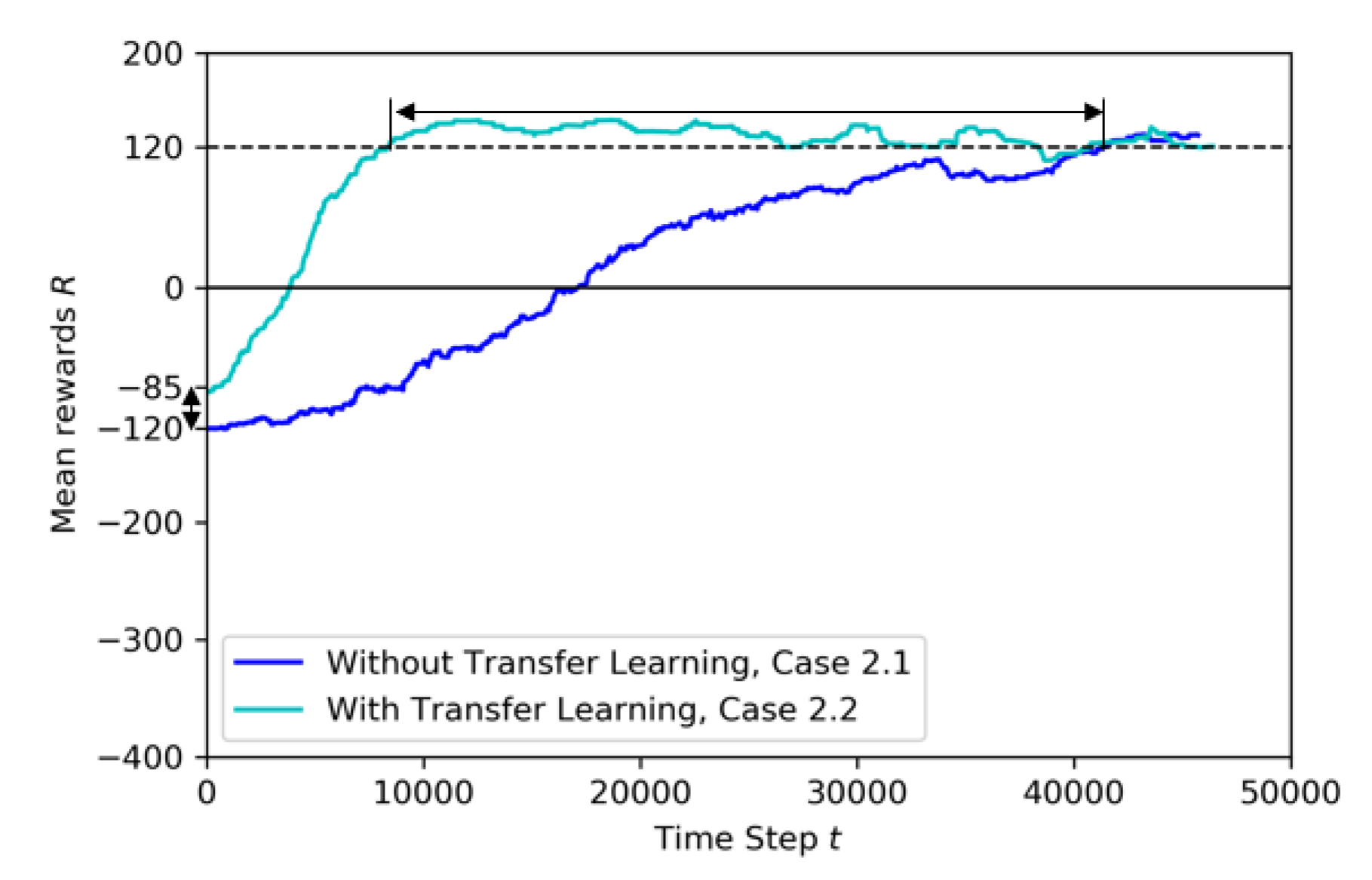
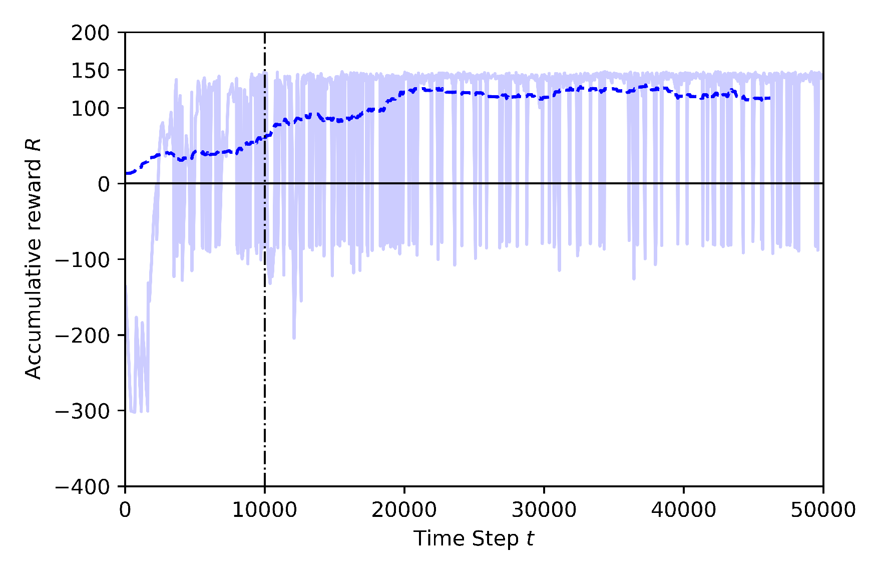
4.3.2. Case 2: Training at Low Altitude, with Many Obstacles
- Case 2.1: without Transfer Learning
- Case 2.2: with Transfer Learning, using pre-trained model from Baseline
5. Further Model Results and Discussion
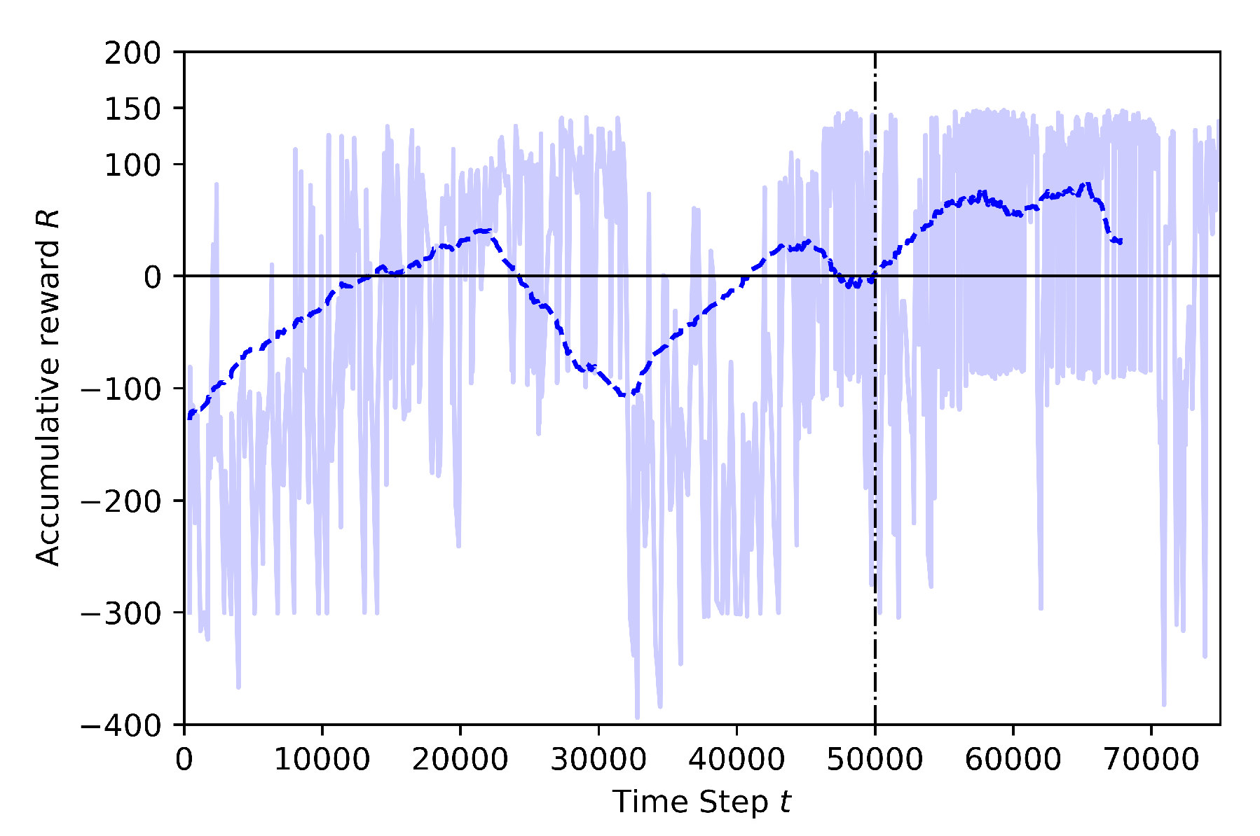
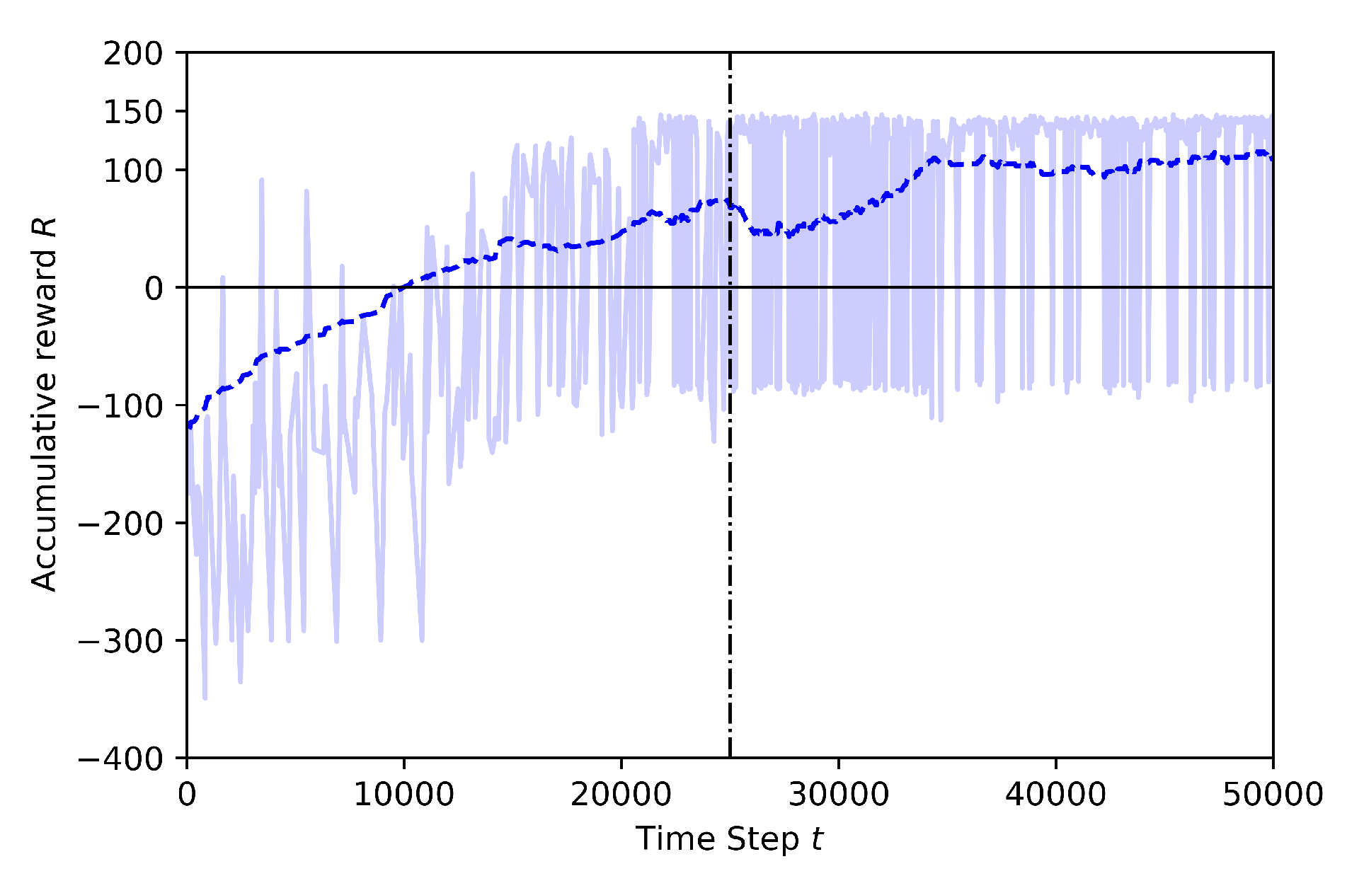
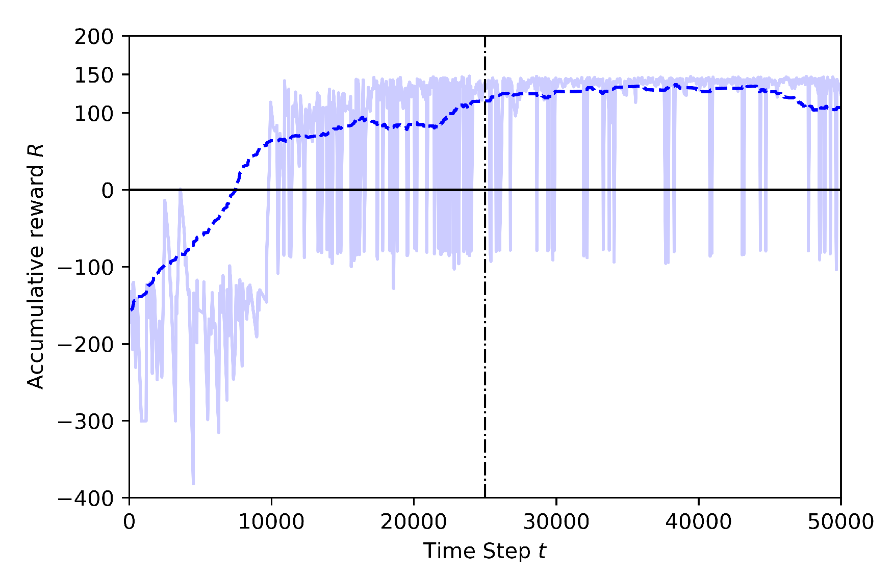
5.1. Comparison of the Effects of Different Annealing Points in TL
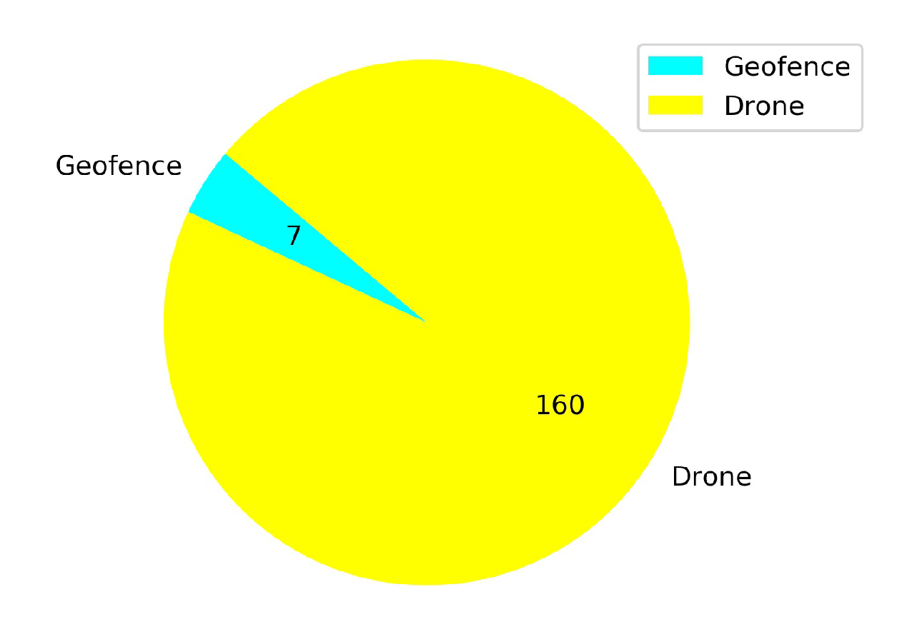
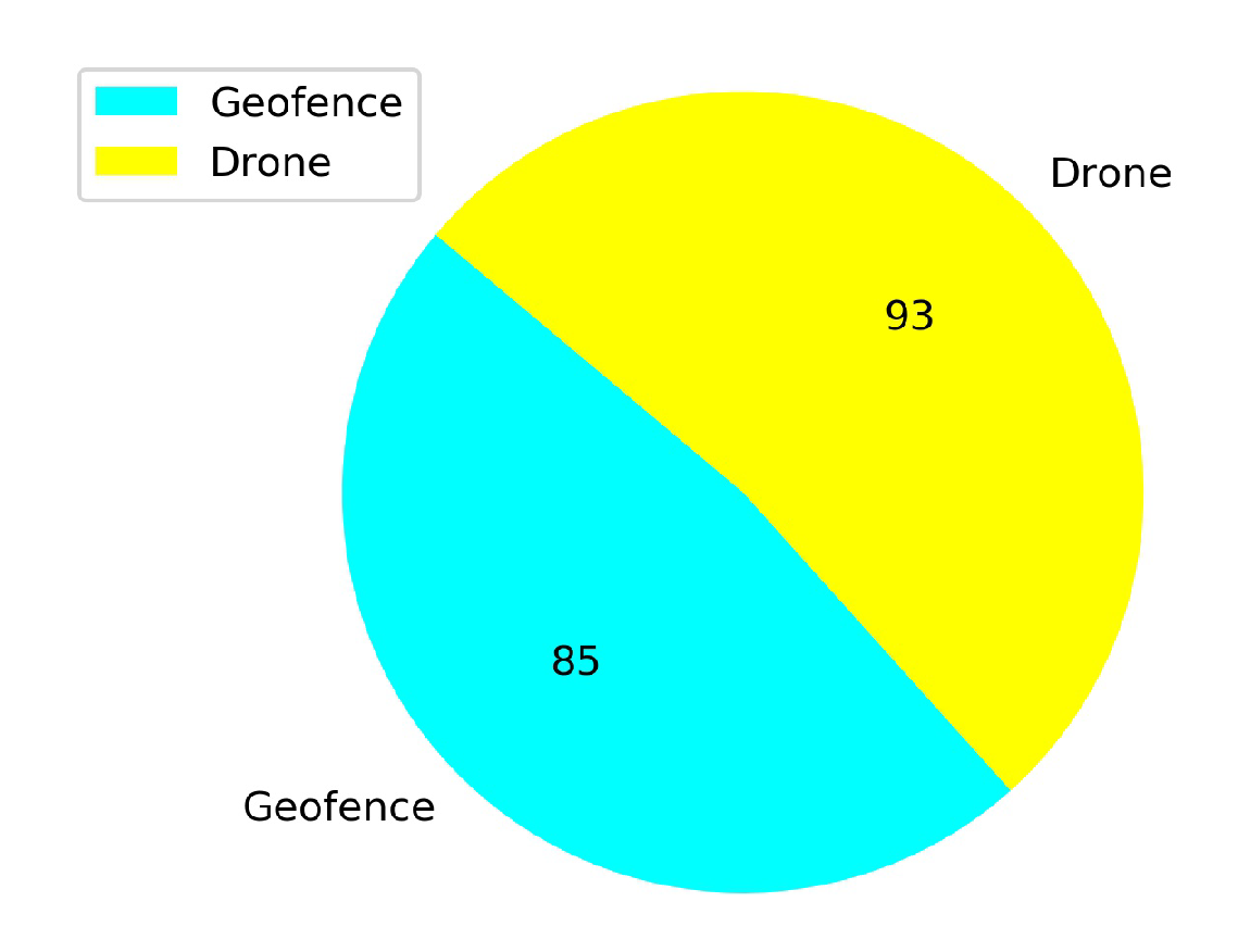
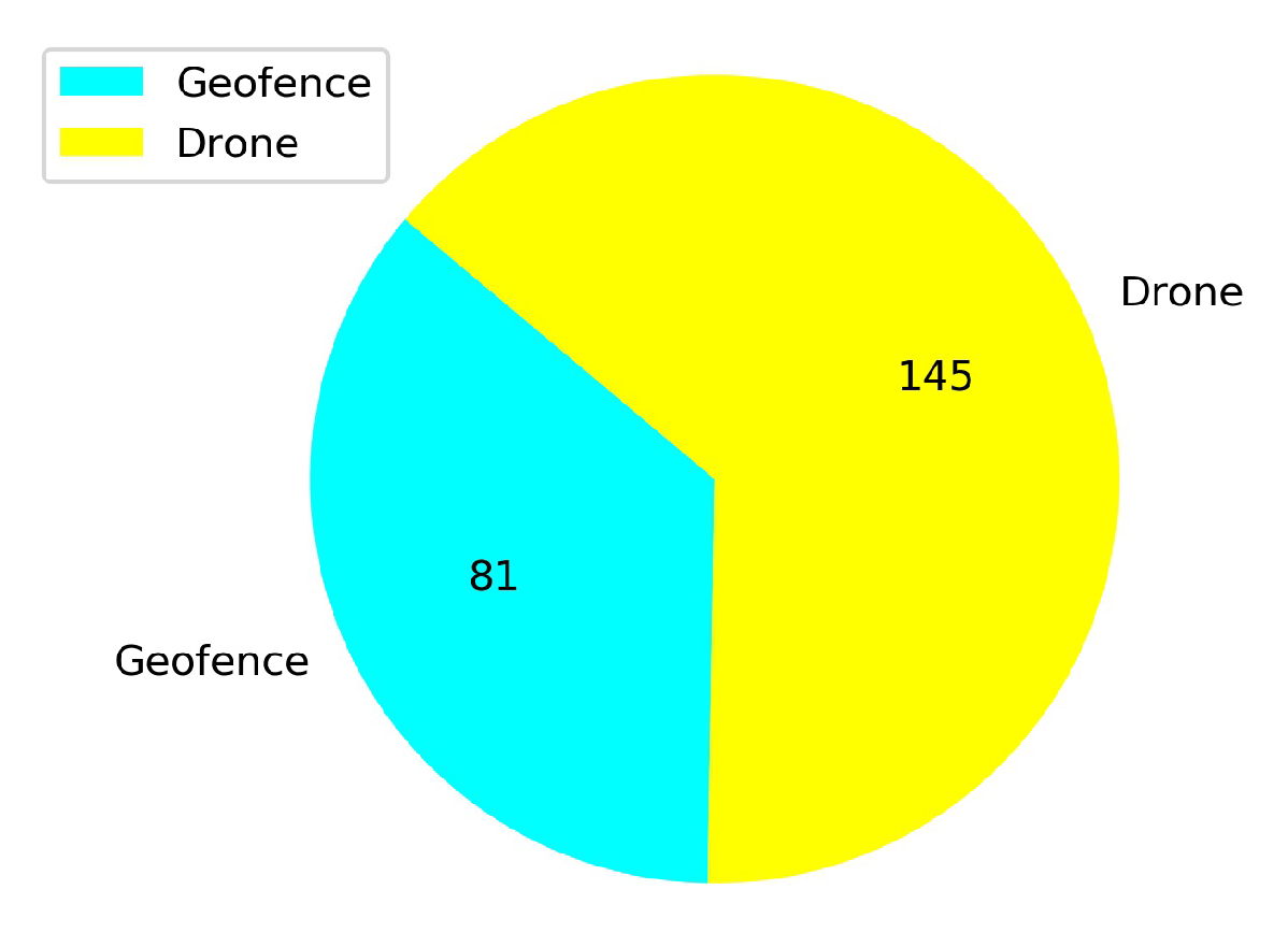
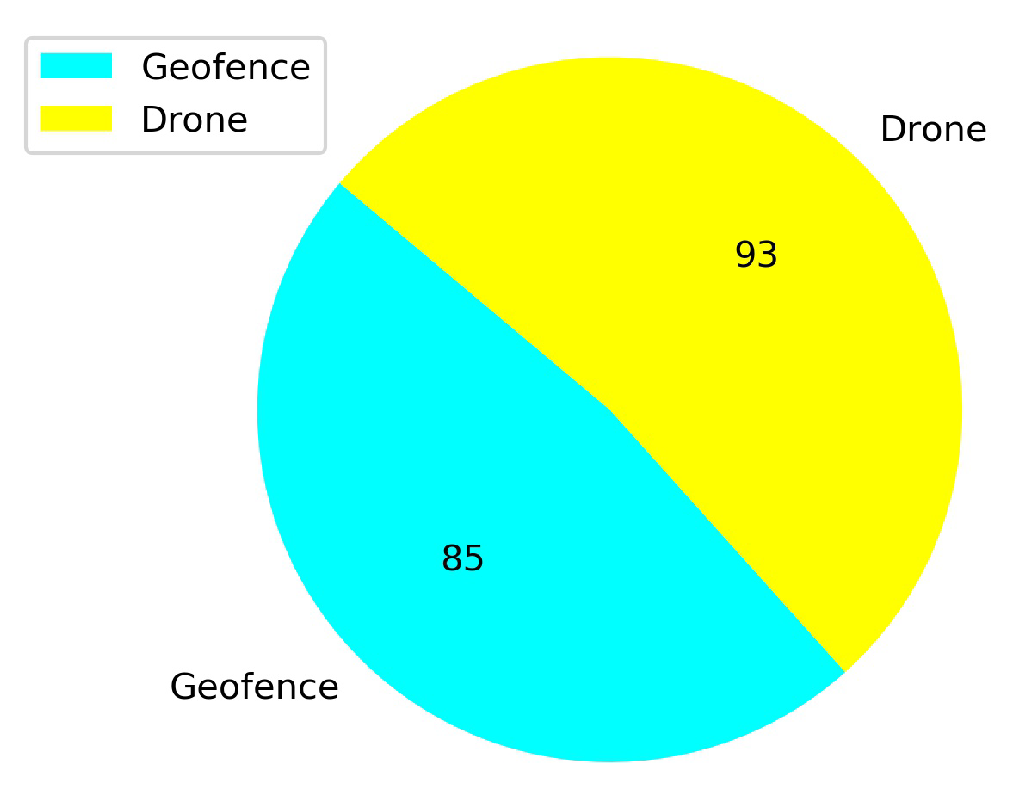
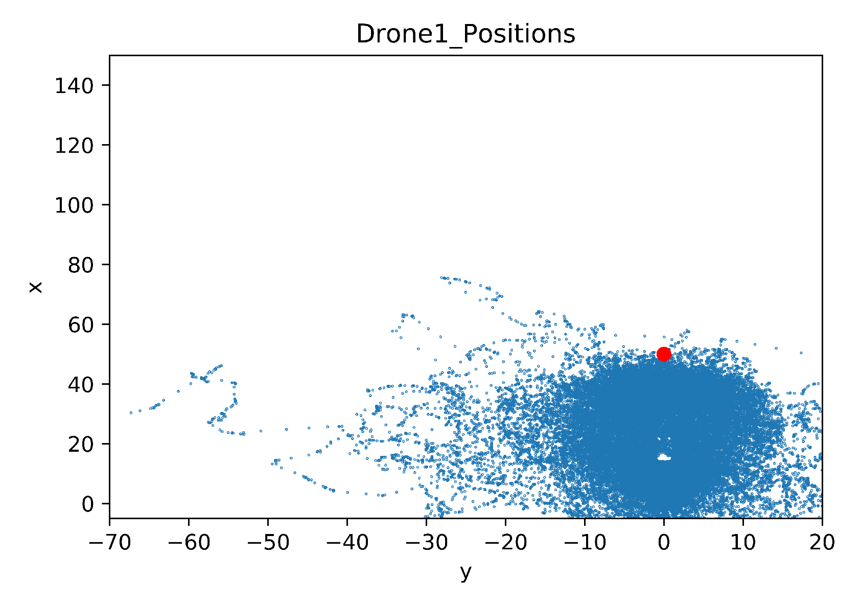
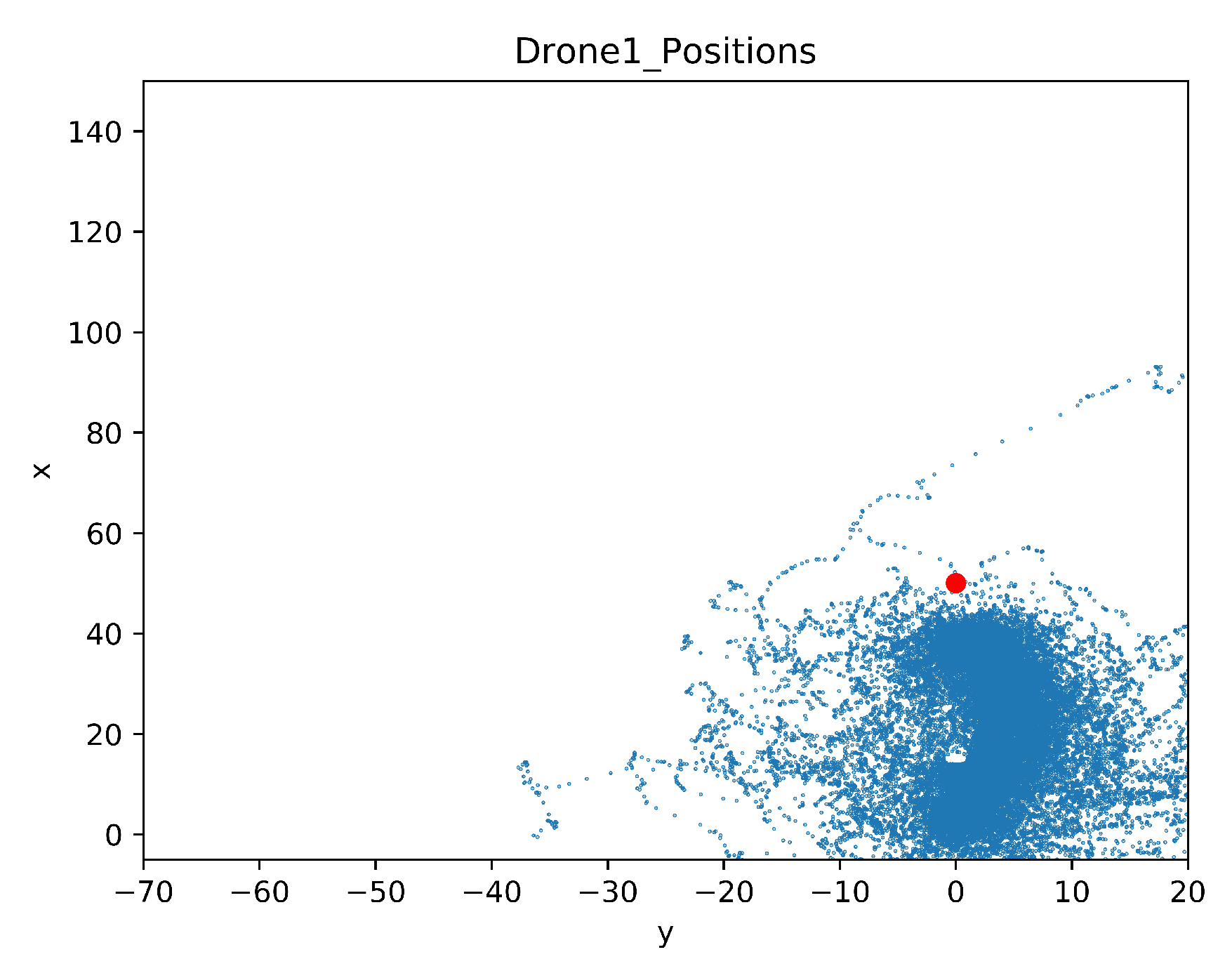
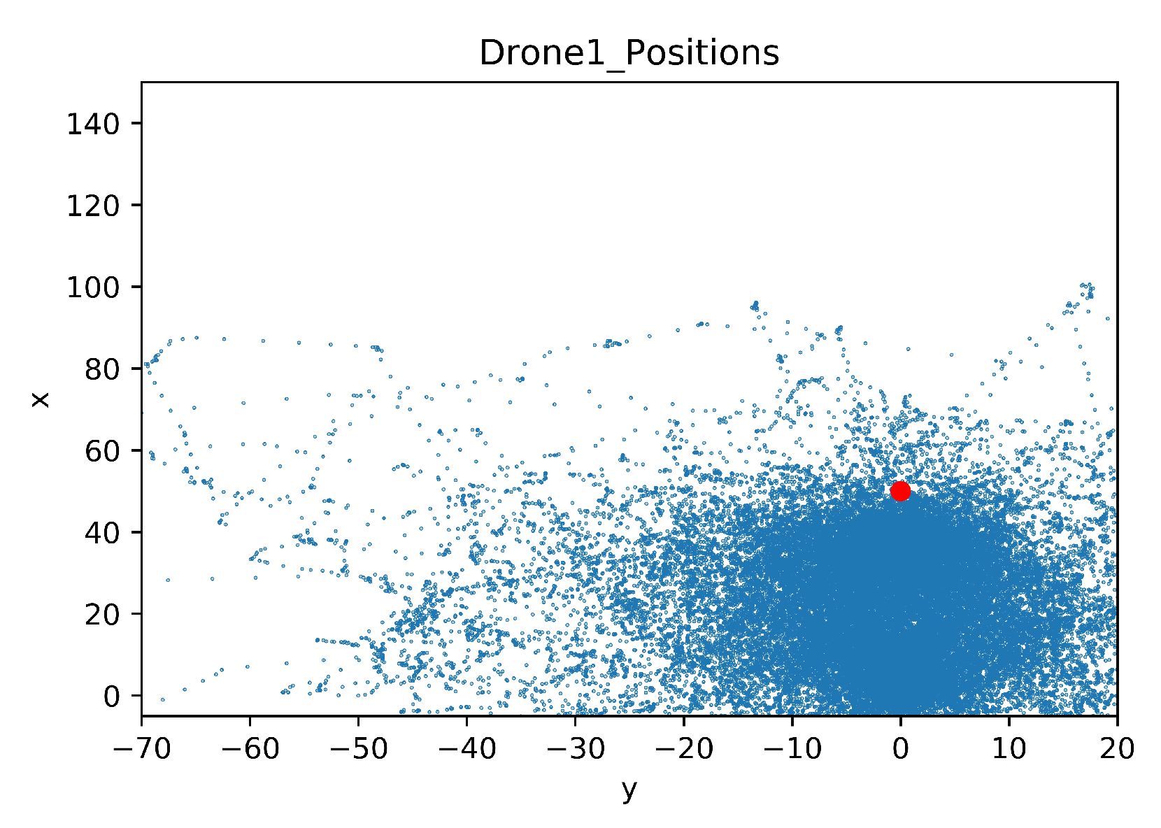
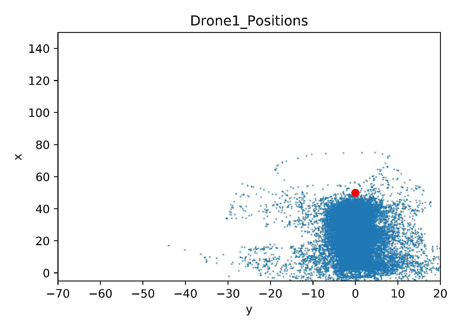
5.2. Comparison of the Explored Areas with or without TL
5.3. Testing the Models at Low Altitude
6. Conclusions
Author Contributions
Funding
Conflicts of Interest
Abbreviations
| UAV | Unmanned Aerial Vehicle |
| AI | Artificial Intelligence |
| DRL | Deep Reinforcement Learning |
| CNN | Convolutional Neural Network |
| RL | Reinforcement Learning |
| TL | Transfer Learning |
| NED | North East Down |
| BVLOS | Beyond Visual Line of Sight |
| ApI | Application Programming Interface |
Appendix A. Neural Network Parameters

References
- European ATM Master Plan: Roadmap for the Safe Integration of Drones into All Classes of Airspace. Available online: https://www.sesarju.eu/node/2993 (accessed on 26 May 2019).
- Fabra, F.; Zamora, W.; Sangüesa, J.; Calafate, C.T.; Cano, J.C.; Manzoni, P. A Distributed Approach for Collision Avoidance between Multirotor UAVs Following Planned Missions. Sensors 2019, 19, 2404. [Google Scholar] [CrossRef] [PubMed]
- Flights Diverted after Gatwick Airport. Available online: https://www.bbc.com/news/uk-england-sussex-48086013 (accessed on 23 August 2019).
- Kratky, M.; Farlik, J. Countering UAVs—The Mover of Research in Military Technology. Def. Sci. J. 2018, 68, 460–466. [Google Scholar] [CrossRef]
- Michel, A.H. Counter-Drone Systems; Center for the Study of the Drone at Bard College. 2018. Available online: https://dronecenter.bard.edu/counter-drone-systems (accessed on 17 April 2020).
- Akhloufi, M.A.; Arola, S.; Bonnet, A. Drones Chasing Drones: Reinforcement Learning and Deep Search Area Proposal. Drones 2019, 3, 58. [Google Scholar] [CrossRef]
- Redmon, J.; Divvala, S.; Girshick, R.; Farhadi, A. You only look once: Unified, real-time object detection. In Proceedings of the IEEE Conference on Computer Vision and Pattern Recognition (CVPR), Las Vegas, NV, USA, 27–30 June 2016; pp. 779–788. [Google Scholar]
- Anwar, A.; Raychowdhury, A. Autonomous Navigation via Deep Reinforcement Learning for Resource Constraint Edge Nodes using Transfer Learning. arXiv 2019, arXiv:1910.05547. [Google Scholar] [CrossRef]
- Unreal Engine 4. Available online: https://www.unrealengine.com/en-US/what-is-unreal-engine-4 (accessed on 29 January 2019).
- Kouris, A.; Bouganis, C.S. Learning to Fly by MySelf: A Self-Supervised CNN-based Approach for Autonomous Navigation. In Proceedings of the 2018 IEEE/RSJ International Conference on Intelligent Robots and Systems (IROS), Madrid, Spain, 1–5 October 2018; pp. 1–9. [Google Scholar]
- Lu, X.; Xiao, L.; Dai, C.; Dai, H. UAV-aided cellular communications with deep reinforcement learning against jamming. arXiv 2018, arXiv:1805.06628. [Google Scholar]
- Rodriguez-Ramos, A.; Sampedro, C.; Bavle, H.; De La Puente, P.; Campoy, P. A deep reinforcement learning strategy for UAV autonomous landing on a moving platform. J. Intell. Robot. Syst. 2019, 93, 351–366. [Google Scholar] [CrossRef]
- Sutton, R.S.; Barto, A.G. Reinforcement Learning: An Introduction; MIT Press Cambridge: London, UK, 1998. [Google Scholar]
- Kiumarsi, B.; Vamvoudakis, K.G.; Modares, H.; Lewis, F.L. Optimal and autonomous control using reinforcement learning: A survey. IEEE Trans. Neural Netw. Learn. Syst. 2018, 29, 2042–2062. [Google Scholar] [CrossRef] [PubMed]
- Mnih, V.; Kavukcuoglu, K.; Silver, D.; Rusu, A.A.; Veness, J.; Bellemare, M.G.; Graves, A.; Riedmiller, M.; Fidjeland, A.K.; Ostrovski, G.; et al. Human-level control through deep reinforcement learning. Nature 2015, 518, 529. [Google Scholar] [CrossRef] [PubMed]
- Mnih, V.; Kavukcuoglu, K.; Silver, D.; Graves, A.; Antonoglou, I.; Wierstra, D.; Riedmiller, M.A. Playing Atari with Deep Reinforcement Learning. arXiv 2013, arXiv:1312.5602. [Google Scholar]
- Van Hasselt, H.; Guez, A.; Silver, D. Deep Reinforcement Learning with Double Q-Learning. In Proceedings of the Thirtieth AAAI Conference on Artificial Intelligence, Phoenix, AZ, USA, 12–17 February 2016. [Google Scholar]
- McClelland, J.L.; Mcnaughton, B.L.; O’Reilly, R.C. Why there are complementary learning systems in the hippocampus and neocortex: Insights from the successes and failures of connectionist models of learning and memory. Psychol. Rev. 1995, 102, 419–457. [Google Scholar] [CrossRef] [PubMed]
- Riedmiller, M. Neural fitted Q iteration-first experiences with a data efficient neural reinforcement learning method. In Proceedings of the 16th European Conference on Machine Learning, Porto, Portugal, 3–7 October 2005; pp. 317–328. [Google Scholar]
- Lin, L.J. Reinforcement Learning for Robots Using Neural Networks. Ph.D. Thesis, Carnegie-Mellon University, Pittsburgh, PA, USA, 6 January 1993. [Google Scholar]
- Hasselt, H.V. Double Q-learning. In Proceedings of the Advances in Neural Information Processing Systems 23: 24th Annual Conference on Neural Information Processing Systems 2010, Vancouver, BC, Canada, 6–9 December 2010; pp. 2613–2621. [Google Scholar]
- Kersandt, K. Deep Reinforcement Learning as Control Method for Autonomous UAVs. Master’s Thesis, Universitat Politècnica de Catalunya, Barcelona, Spain, 2017. [Google Scholar]
- Taylor, M.E.; Stone, P. Transfer learning for reinforcement learning domains: A survey. J. Mach. Learn. Res. 2009, 10, 1633–1685. [Google Scholar]
- Shah, S.; Dey, D.; Lovett, C.; Kapoor, A. AirSim: High-Fidelity Visual and Physical Simulation for Autonomous Vehicles. In Field and Service Robotics; Springer: Cham, Switzerland, 2017; pp. 621–635. [Google Scholar]
- Brockman, G.; Cheung, V.; Pettersson, L.; Schneider, J.; Schulman, J.; Tang, J.; Zaremba, W. OpenAI Gym 2016. Available online: https://arxiv.org/abs/1606.01540 (accessed on 17 April 2020).
- Abadi, M.; Agarwal, A.; Barham, P.; Brevdo, E.; Chen, Z.; Citro, C.; Corrado, G.S.; Davis, A.; Dean, J.; Devin, M.; et al. TensorFlow: Large-Scale Machine Learning on Heterogeneous Distributed Systems. arXiv 2015, arXiv:1603.04467. [Google Scholar]
- Theano Development Team. Theano: A Python framework for fast computation of mathematical expressions. arXiv 2016, arXiv:1605.02688.
- Plappert, M. keras-rl. Available online: https://github.com/keras-rl/keras-rl (accessed on 17 April 2020).
- Von Bothmer, F. Missing Man: Contextualising Legal Reviews for Autonomous Weapon Systems. Ph.D. Thesis, Universität St. Gallen, St. Gallen, Switzerland, May 2018. [Google Scholar]
- Gurriet, T.; Ciarletta, L. Towards a generic and modular geofencing strategy for civilian UAVs. In Proceedings of the 2016 International Conference on Unmanned Aircraft Systems (ICUAS), Arlington, VA, USA, 7–10 June 2016; pp. 540–549. [Google Scholar]
- AirSim Documentation. Available online: https://microsoft.github.io/AirSim (accessed on 1 May 2019).
- Samek, W.; Wiegand, T.; Müller, K.R. Explainable Artificial Intelligence: Understanding, Visualizing and Interpreting Deep Learning Models. arXiv 2018, arXiv:1708.08296. [Google Scholar]


| Method Type | The Number of Cases Available |
|---|---|
| Jamming | 96 |
| Net | 18 |
| Spoofing | 12 |
| Laser | 12 |
| Machine Gun | 3 |
| Electromagnetic Pulse | 2 |
| Water Projector | 1 |
| Sacrificial Collision Drone | 1 |
| Other | 6 |
| Reward | The Reason |
|---|---|
| +100 | Goal reached |
| −100 | Collision: Obstacle (stationary or moving) or geofence |
| −1 + Distance + TrackAngle | Otherwise |
| Case | Training | Steps | Annealing | Geofence | Obstacles |
|---|---|---|---|---|---|
| Baseline | FULL | 125K | 50K | YES | NONE |
| Case 1.1 | FULL | 75K | 50K | YES | stationary 3rd drone |
| Case 1.2 | Transferred | 50K | 25K | YES | stationary 3rd drone |
| Case 1.3 | FULL | 75K | 50K | YES | non-stationary 3rd drone |
| Case 1.4 | Transferred | 50K | 25K | YES | non-stationary 3rd drone |
| Case 2.1 | FULL | 125K | 50K | YES | houses, trees, electrical, etc. |
| Case 2.2 | Transferred | 50K | 10K | YES | houses, trees, electrical, etc. |
© 2020 by the authors. Licensee MDPI, Basel, Switzerland. This article is an open access article distributed under the terms and conditions of the Creative Commons Attribution (CC BY) license (http://creativecommons.org/licenses/by/4.0/).
Share and Cite
Çetin, E.; Barrado, C.; Pastor, E. Counter a Drone in a Complex Neighborhood Area by Deep Reinforcement Learning. Sensors 2020, 20, 2320. https://doi.org/10.3390/s20082320
Çetin E, Barrado C, Pastor E. Counter a Drone in a Complex Neighborhood Area by Deep Reinforcement Learning. Sensors. 2020; 20(8):2320. https://doi.org/10.3390/s20082320
Chicago/Turabian StyleÇetin, Ender, Cristina Barrado, and Enric Pastor. 2020. "Counter a Drone in a Complex Neighborhood Area by Deep Reinforcement Learning" Sensors 20, no. 8: 2320. https://doi.org/10.3390/s20082320
APA StyleÇetin, E., Barrado, C., & Pastor, E. (2020). Counter a Drone in a Complex Neighborhood Area by Deep Reinforcement Learning. Sensors, 20(8), 2320. https://doi.org/10.3390/s20082320