1. Introduction
Deformation monitoring can reveal unstable slope surfaces to prevent serious safety hazards. It is deployed to determine changes in the shape and displacements of a deformable body in temporal and spatial domains [
1]. Advancements in signal processing, integrated circuit, microwave, and antenna technologies have made synthetic aperture radar (SAR) a notable innovation in the radar technology field. Interferometry is a technique for extracting deformation information by comparing the observed phases before and after the deformation of an object. SAR interferometry technology can be used for all-weather situations and the high-precision monitoring of ground surface deformations across large areas [
2]. Ground-based synthetic aperture radar interferometry (GB-InSAR) has been tested in various fields in recent years including the monitoring of landslides, open-pit mines, ground subsidence, architectural structures, bridges, sinkholes, and glacier displacements [
3,
4,
5,
6,
7,
8]. Despite these achievements, there are yet obstacles hindering the practical application of GB-InSAR deformation monitoring. Traditional SAR can obtain 2D images in steep and complex terrain, but 3D objects may be severe distorted on the 2D image which obscures several targets [
9,
10,
11]. SAR sensors can resolve different monitored targets based on their slant ranges from the targets to the radar center and the angles away from the centerline of the radar antenna middle beam. Unlike the orthographic projection of a traditional topographic map and the central projection of photogrammetry, SAR-based image projection generally requires manual interpretation to identify a deformed target and its position in the planar coordinate system of a radar image. The interpretation of radar images requires understanding and judgment of radar observation geometry and imaging principles, matching with 3D scenes, and accurately locating deformation areas and variations. The analyst must have sufficient knowledge to ensure appropriate such identifications. The issue of accurately interpreting 3D measurement results is key regarding successful GB-InSAR implementation.
Previous research has explored GB-InSAR mapping technology in the GB-InSAR geometric mapping context. Tapet et al., for example, integrated terrestrial laser scanning (TLS) and GB-InSAR to monitor heritage building deformations and accurately located deformed areas [
5]. Yue et al. fused GB-radar and survey robot data to determine the spatial relationship between the robot monitored 3D deformations and the GB-radar coordinate system [
12]. The method was used for 1D deformation and was not expanded in high dimensions. GB-InSAR and InSAR have unique observation geometry and measurement modes, so applying the InSAR processing method to GB-InSAR produces a substantial error. The integration of high-precision external auxiliary measurements may be an effective solution to this problem. Zou, of Wuhan University, fused ground-based SAR and 3D laser scanning data for the 3D visualization of GB-InSAR in a hydro-dam deformation monitoring experiment using point cloud, coordinate transformation and projection, and 2D four-parameter transformation techniques [
13]. Yang et al. proposed a geometric 3D matching method based on both range and azimuth constraints for frontal and lateral strip SAR and terrain data, [
14]. Wang et al. used 3D laser scanning data to assist the 3D coordinate transformation of GB-InSAR image pixels; they also applied a scaling factor method based on the parameter estimation of a similar transformation. They put forward the idea of mismatching correction based on control points [
9]. In general, inconsistencies among systems, variations in the measurement environment, and scene image changes remain problematic. In an experiment on ground-based SAR deformation monitoring, Yang et al. used a positioning method to determine the rail endpoint coordinate and artificial targets [
4]. Lombardi et al. [
15] integrated GB-InSAR and 3D laser scanning for landslide monitoring. Zheng et al. investigated data fusion and deformation comparison with GB-InSAR and 3D laser scanning in a controlled field test and later they integrated GB-InSAR, TLS and unmanned aerial vehicle photogrammetry (UAV) in a rock slide residual mass emergency monitoring case [
1,
16].
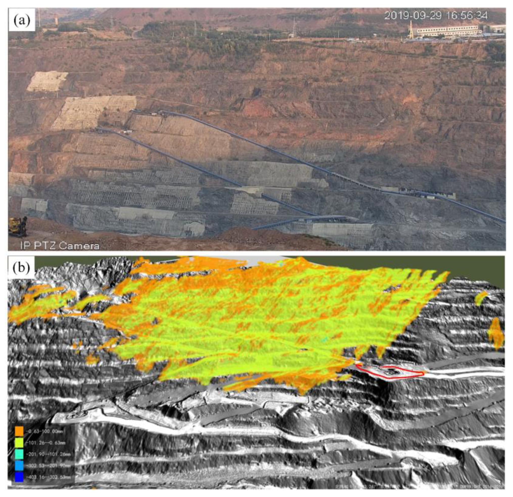
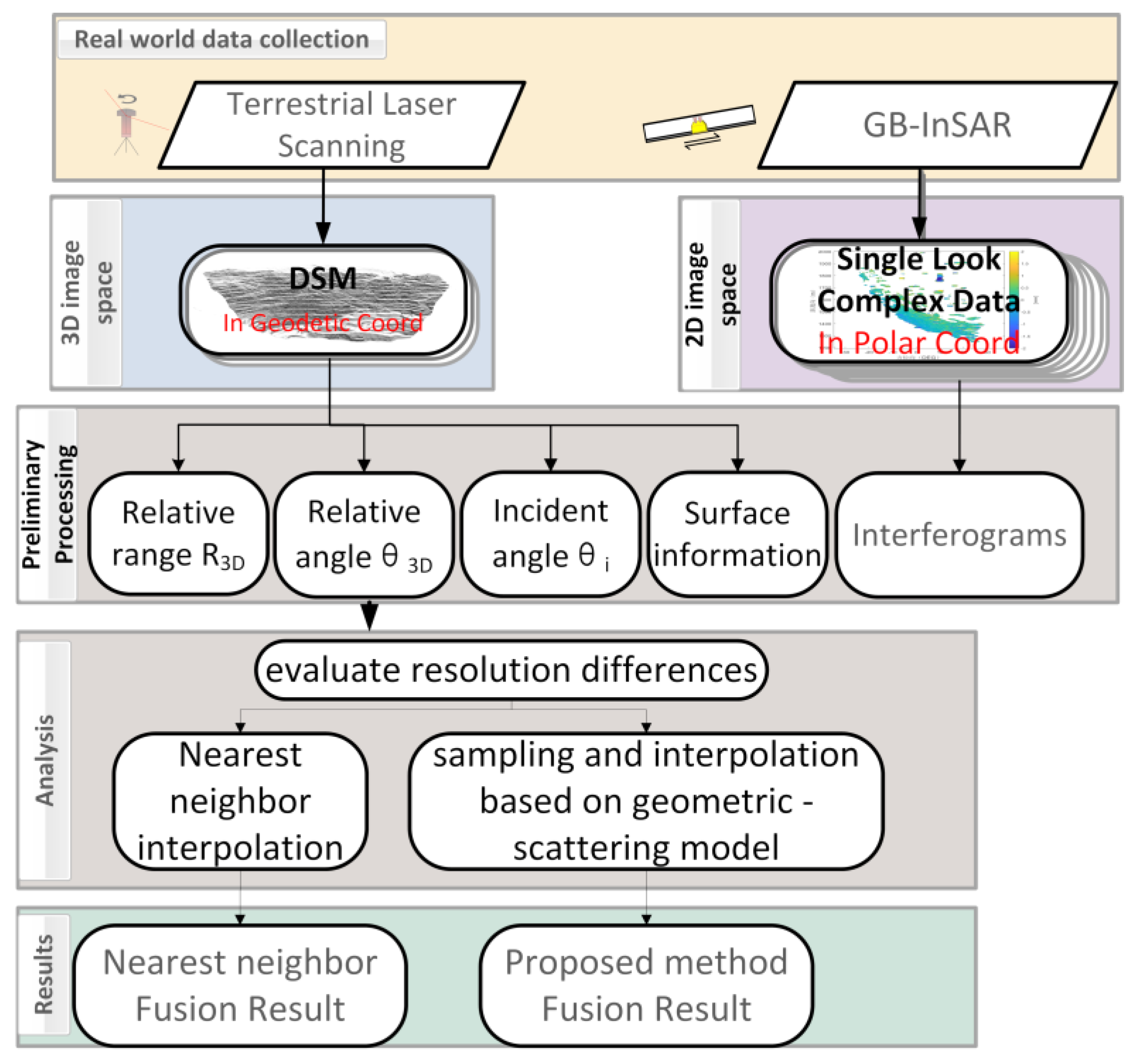
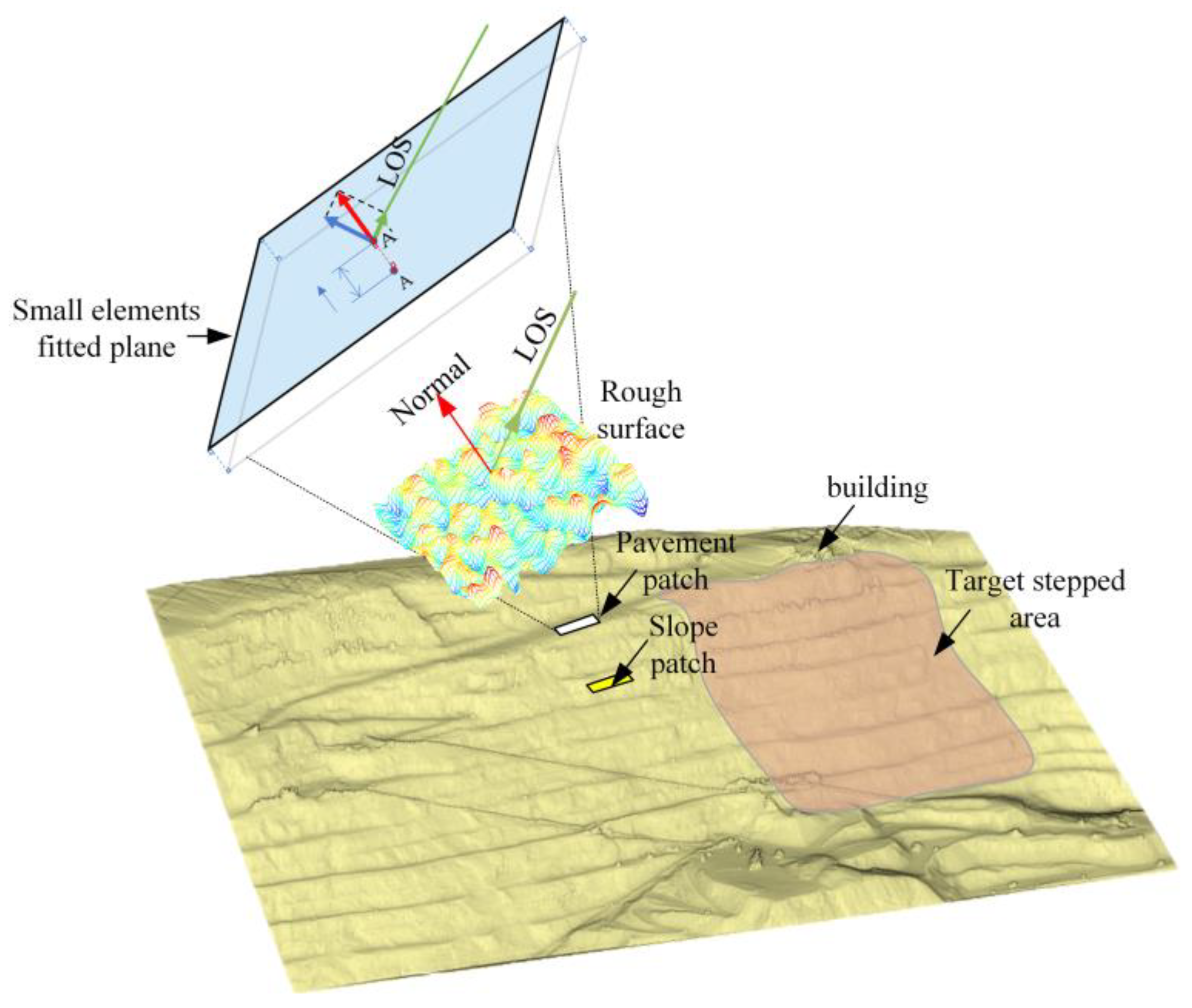
The geometric mapping of the GB-InSAR image and 3D terrain data is an important step in the deformation monitoring process. During a monitoring case in an open-pit mine, we encountered a problem: mapping results cannot differentiate slope steps differences. The problem confused geo-engineers in analyzing the deduction of spatial and temporal deformation patterns. Based on the above analysis, we can conclude that extant geometric mapping methods are deficient in the mapping relation of multiple spatially distributed target points of the radar pixel with the point cloud, as well as the 3D features (e.g., structure, texture, and occlusion) in reflecting targets. The points cloud may help inversion of the scattering difference of GB-InSAR, which would help differentiate the pavement and slope. Conventional mapping methods based on nearest-neighbor interpolation cannot be effectively applied to SAR pixels. Based on the basic cognition that SAR image is a kind of target scattering characteristic difference representation map. We develop a method that is comprised of a geometric mapping and scattering variance weighting model. The model is introduced in setting the interpolation weight of points in one radar pixel. The method may help in identifying shadows and layover in topographically rugged areas.
The paper is organized as follows.
Section 2 discusses the problem we encountered and solving scheme by an improved linear GB-InSAR and TLS data fusion method.
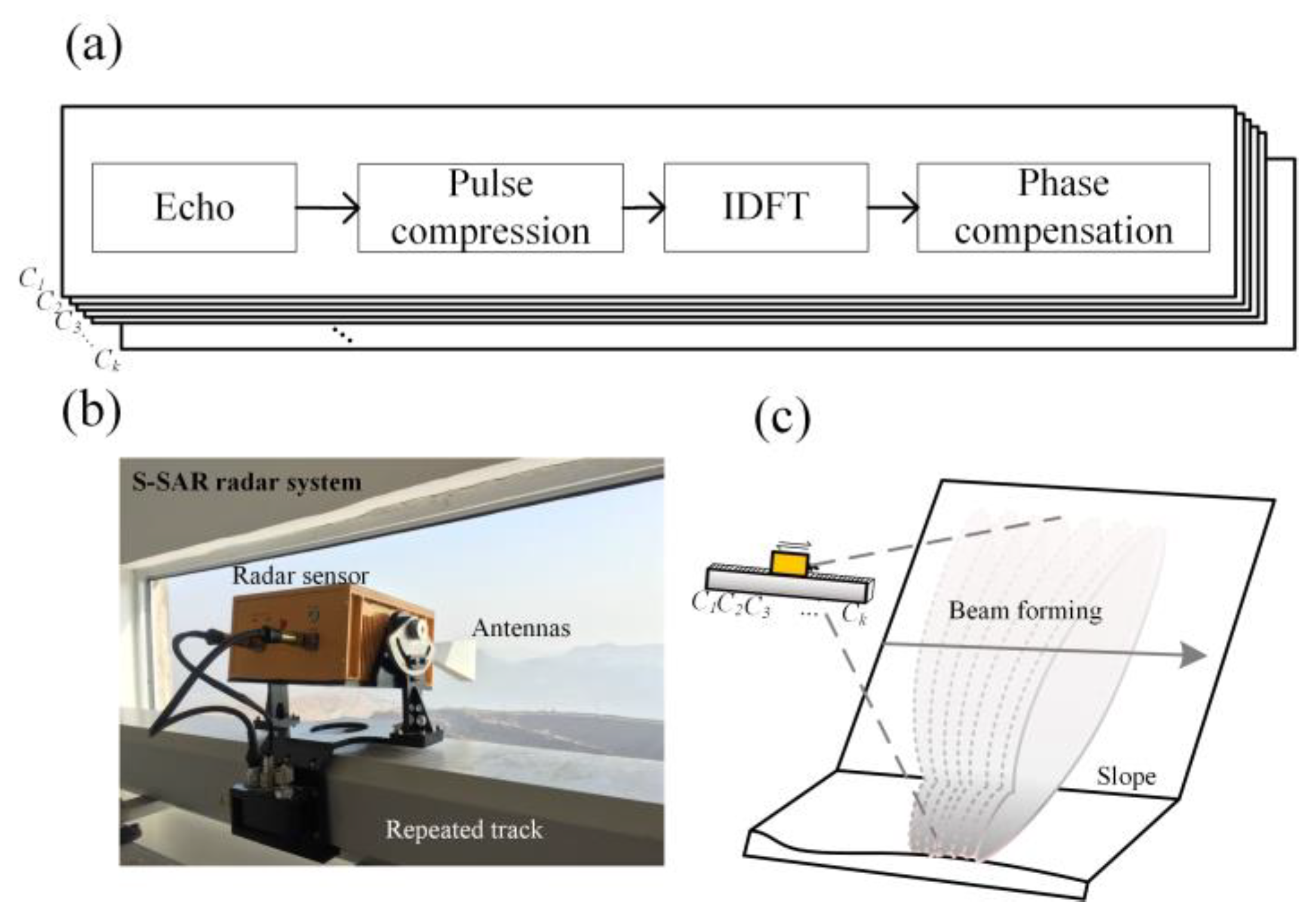
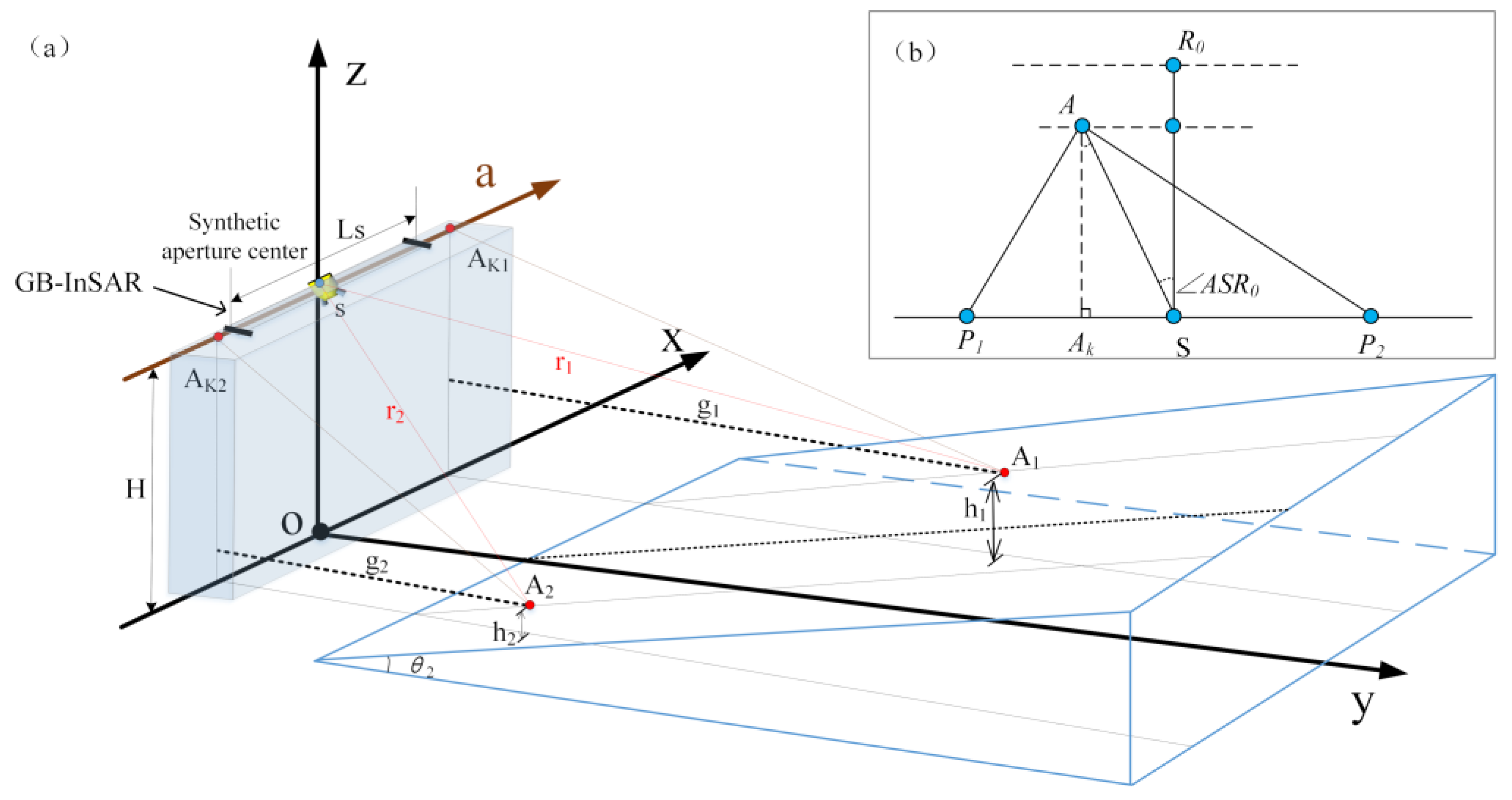
Section 3 further discusses the GB-InSAR system and the rough surface slope topographic data model. The GB-InSAR image and spatial point cloud 3D mapping method, which is based on geometric and scattering models, is also delineated in
Section 3.
Section 4 presents a data fusion experiment in an open-pit mine in China, which was conducted to validate the model.
Section 5 discusses the influence factors and possible solutions.
Section 6 provides a summary and recommendations for future research.
4. Results
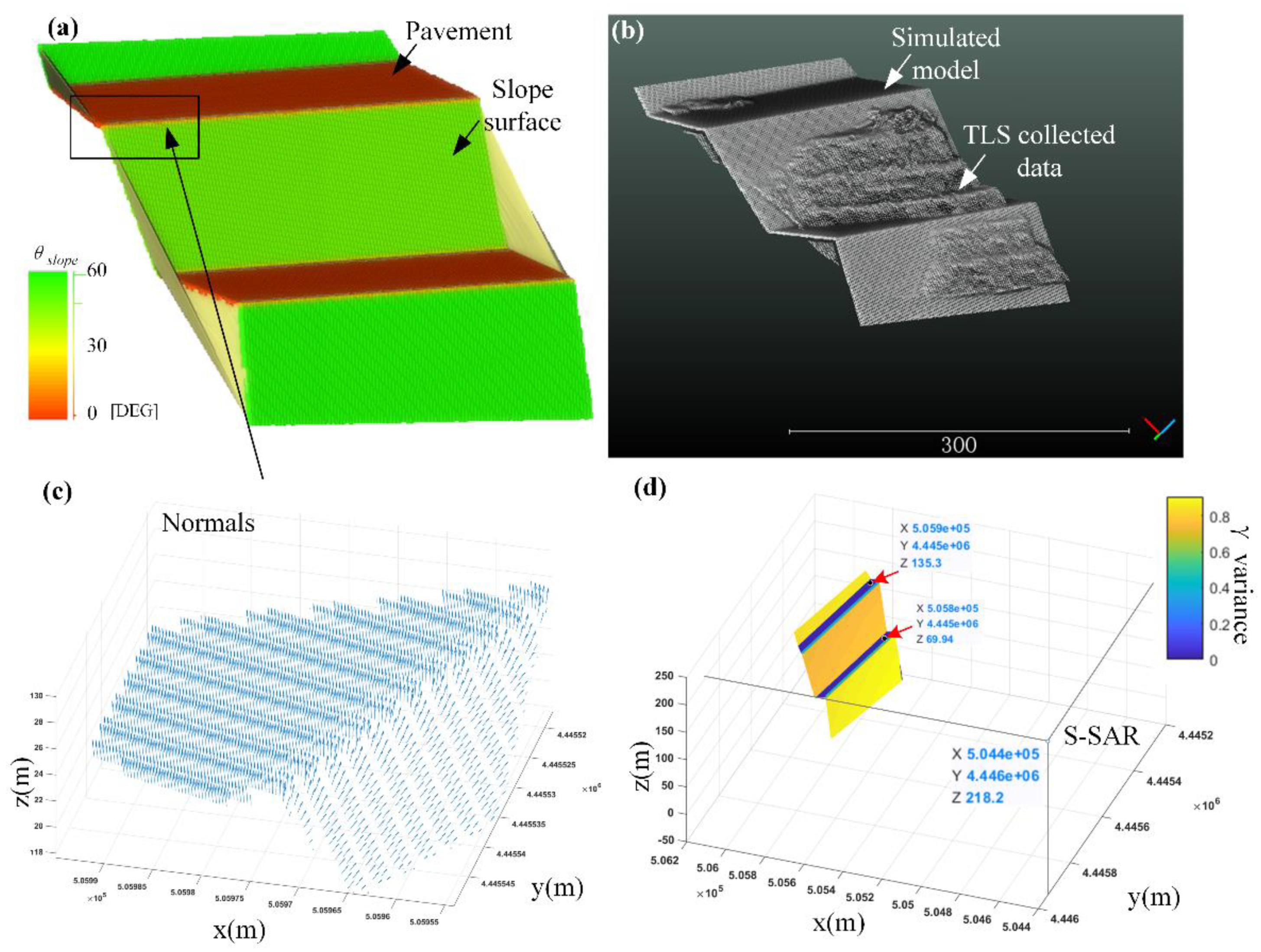
A slope-pavement model was established (
Figure 8a). The step model consists of slope and pavement components. The deformable regions were simulated across the road and slope on a deformation image based on the simulated monitored slope. The nearest-neighbor interpolation method and the proposed method were used separately for mapping to observe whether the projected deformation was consistent with the shape of the step. The model has been geocoded with the target area based on block stretching and linear transformation (
Figure 8b).
Normal
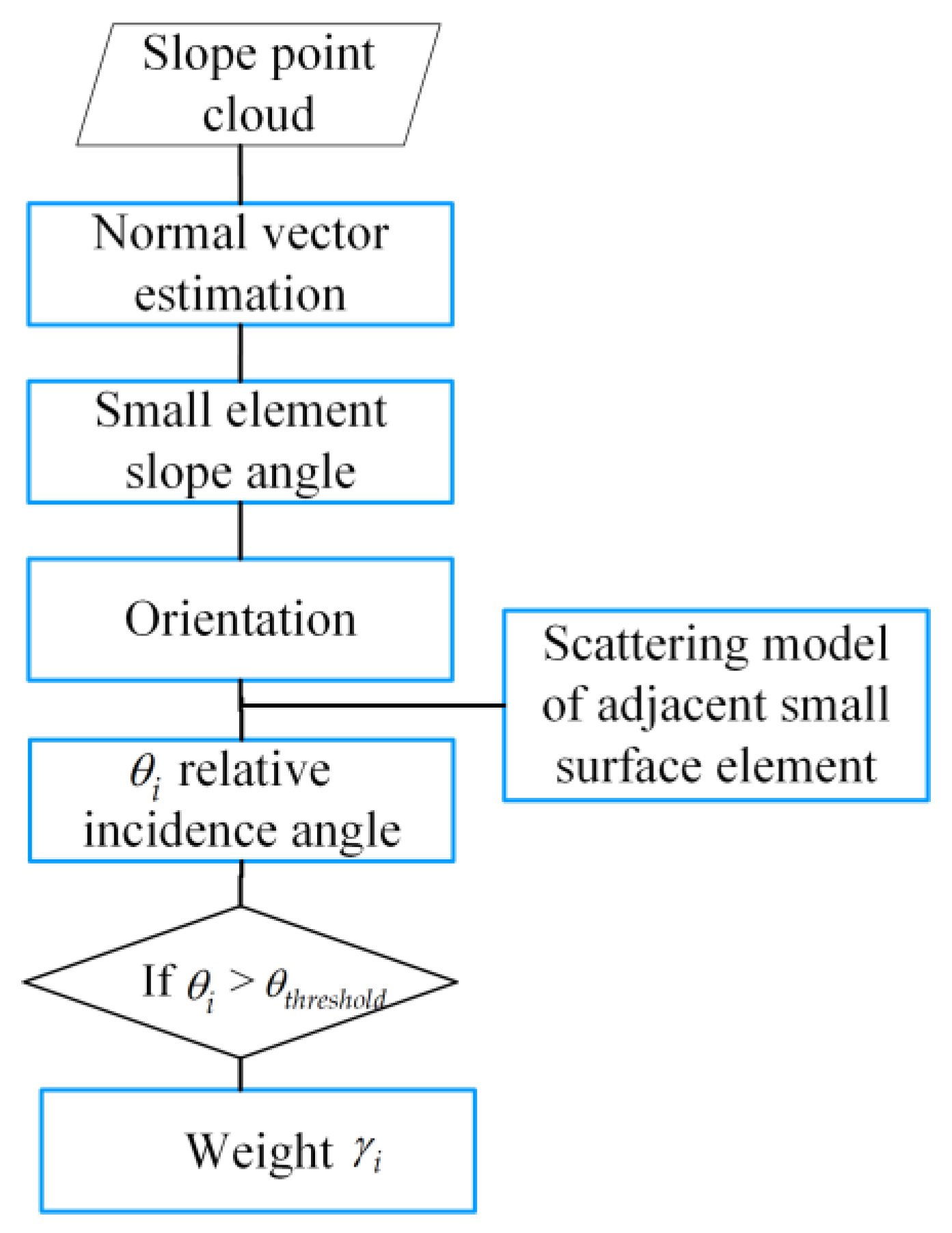
: Normal vector computing is integrated into many point cloud processing software and C++ library, for example: Cloud compare, MeshLab, and point cloud library (PCL). We programmed with the PCL library and referenced the Cloud compare built-in minimum spanning tree method to extract normal vectors of the sampled step model.
is as shown in
Figure 8c. The pavement and the slope can be differentiated by
.
Orientation: The orientation of each point in the model is easy to extract. As the step model coded, it has a certain horizontal coordinate system plane. The angle between and horizontal plane normal can be treated as an orientation vector , and the of each point in Equation (6) is identified.
Line-of-sight (LOS): LOS is the vector that connects each point to radar Station S.
Relative incident angle : can be determined by Equation (11).
Weight
:
is the normalization of
. The result is shown in
Figure 8d.
One rather important thing to note, the simulated stepped model is more like a “smooth surface” consist of many particles. However, the target area in a natural scene is more like a “rough surface”.
Figure 8d shows the weight difference of the stepped model. The pavement weight was much lower than the slope surface through SAR beam incidents in an overlooking perspective. The weight of pavement only means the incident angle is not good, which may lead to a disappearance of deformation in the geometric mapping process. The topographically rugged surface of the pavement will not be affected by the deformation disappearance.
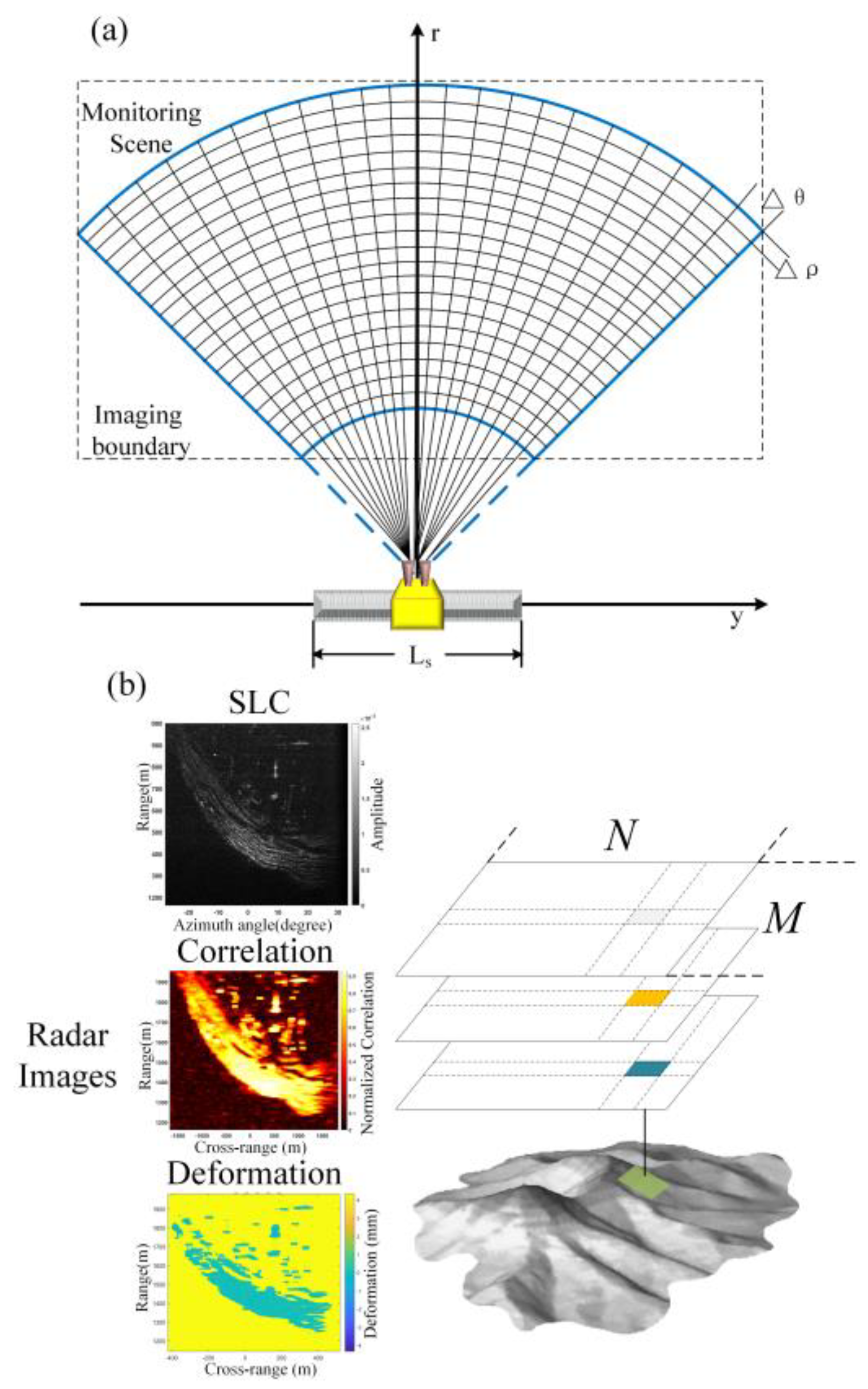
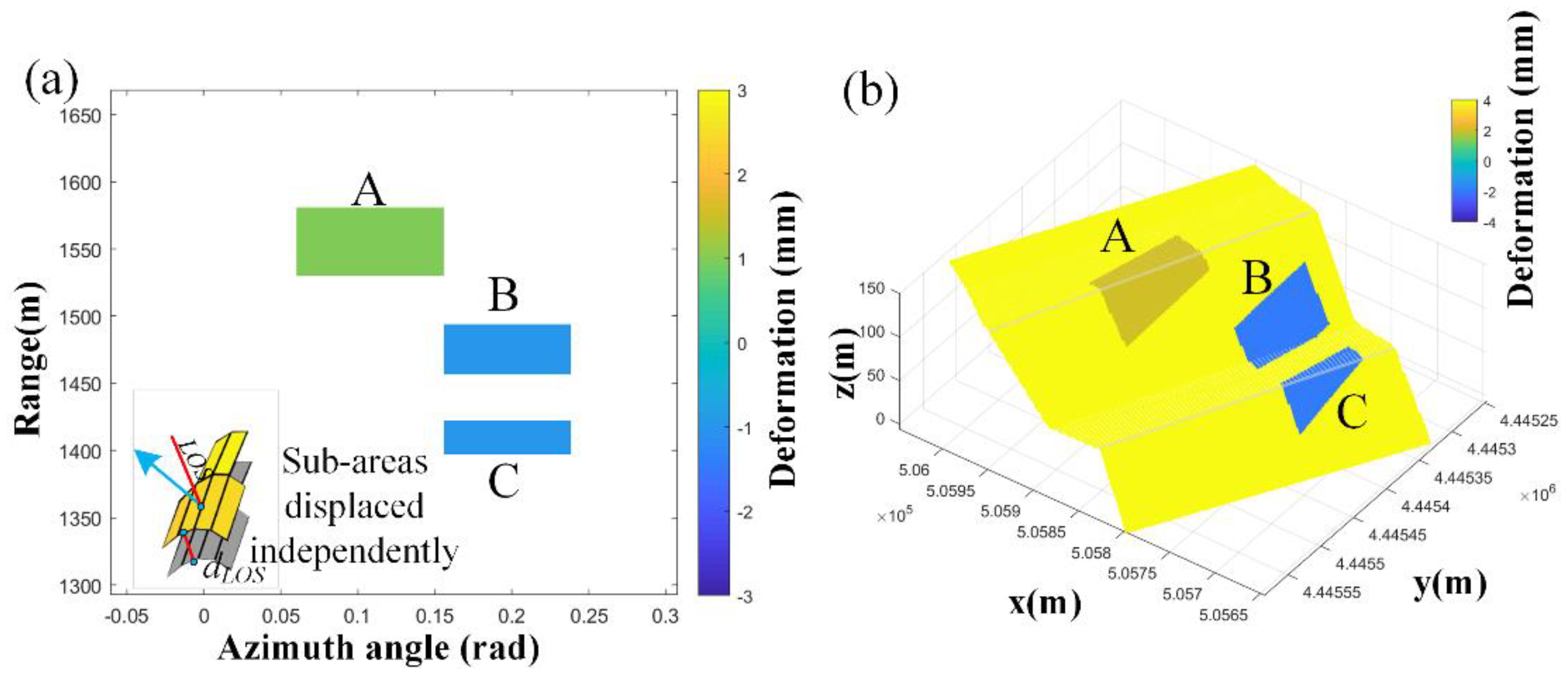
Sub-area deformation positioning: The mapping relation table of the 3D point cloud and radar image was established via geometric mapping. Several subregions were identified in the diagram that are composed of groups of pixels that appear as blocks on the surface. As shown in
Figure 9a, these blocks have a global displacement along the LOS direction; this simulates the displacement detected by the radar rather than changes in the 3D model. The simulation results can then be mapped to a 3D space as shown in
Figure 9b. This case features sub-area overall deformation. The GB-InSAR image as-collected from the open-pit mine was used to match the real terrain point cloud and simulated terrain point cloud using the method described in
Section 2. Several sub-areas that cover the pavement and slope surface were then created as shown in
Figure 9a–c were the index of the sub-area. However, in the real world, the deformation of the road surface and slope surface is always different, so simulation case 1 only shows the spatial positioning of each sub-area.
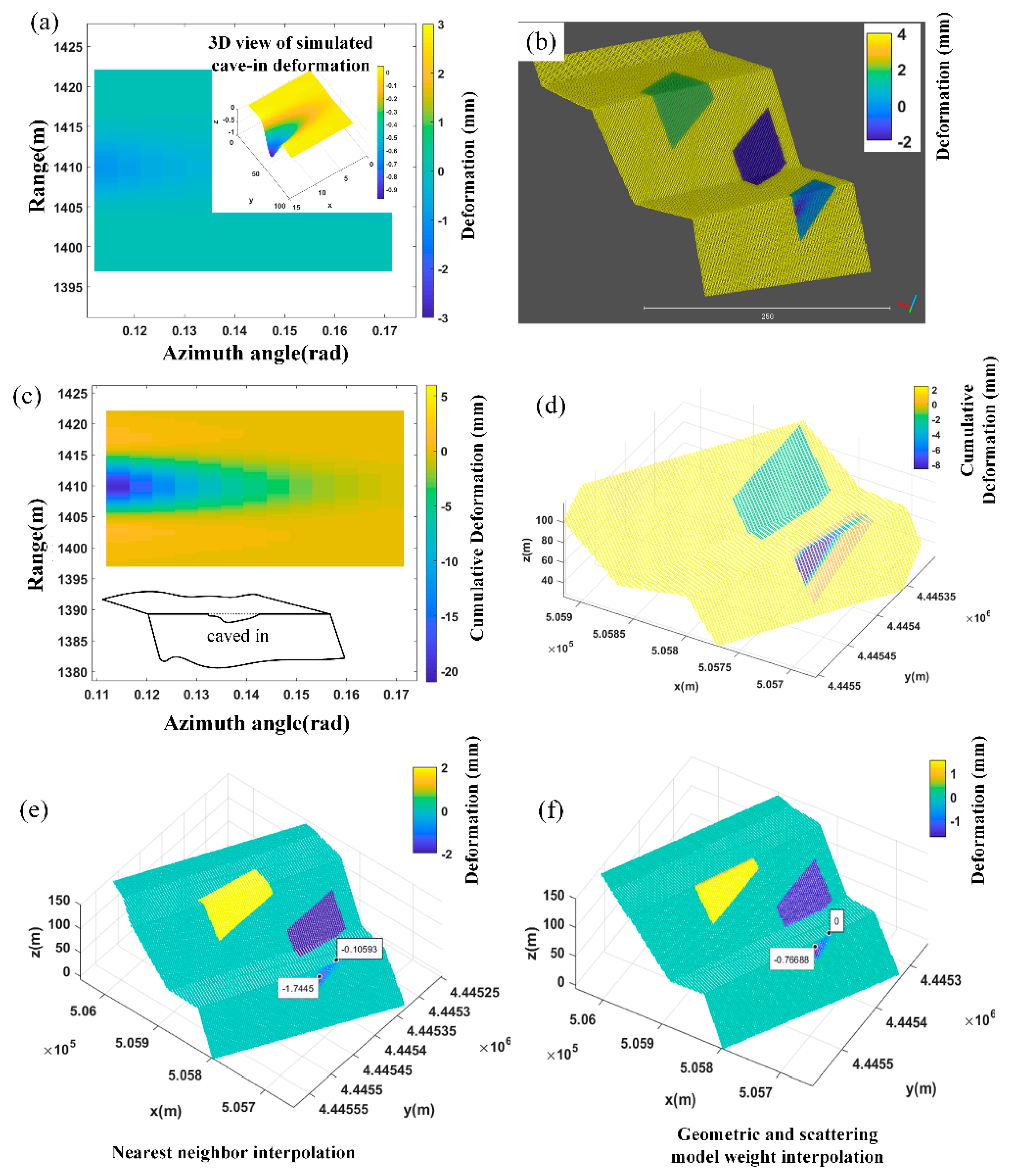
Continuous deformation generated through simulation in Region C: This was a simulation of a slope surface collapse, where the flow of water in the slope was caused by internal empty surface sag. The deformation field was simulated via a quadratic function model, as shown in
Figure 10a. At this point, the lower part of the slope moved down relative to the radar resulting in a negative displacement relative to the radar. This was then projected into 3D space using the nearest-neighbor method (
Figure 10b). If the area produces persistent, identical depressions and is detected by GB-InSAR, then the subsequent deformation image is the same as the image shown in
Figure 10c. Then the deformation values of each pixel can be accumulated to form the image. At this point, there is a gradual and non-linear deterioration of the slope. If a pixel is across the slope and road surface, the assignment of the point cloud within the pixel set should be distinguishable. Scattering model analysis can solve this problem. If the radar wave incident angle of the road is poor but that of the slope is acceptable, then the nearest-neighbor method results of the road surface and slope are the same. The proposed method makes the road result more distinguishable by reducing its weight and strengthening slope results. Based on the above assumptions, the normal vector of each point was calculated followed by the slope angle of the small surface element adjacent to each point.
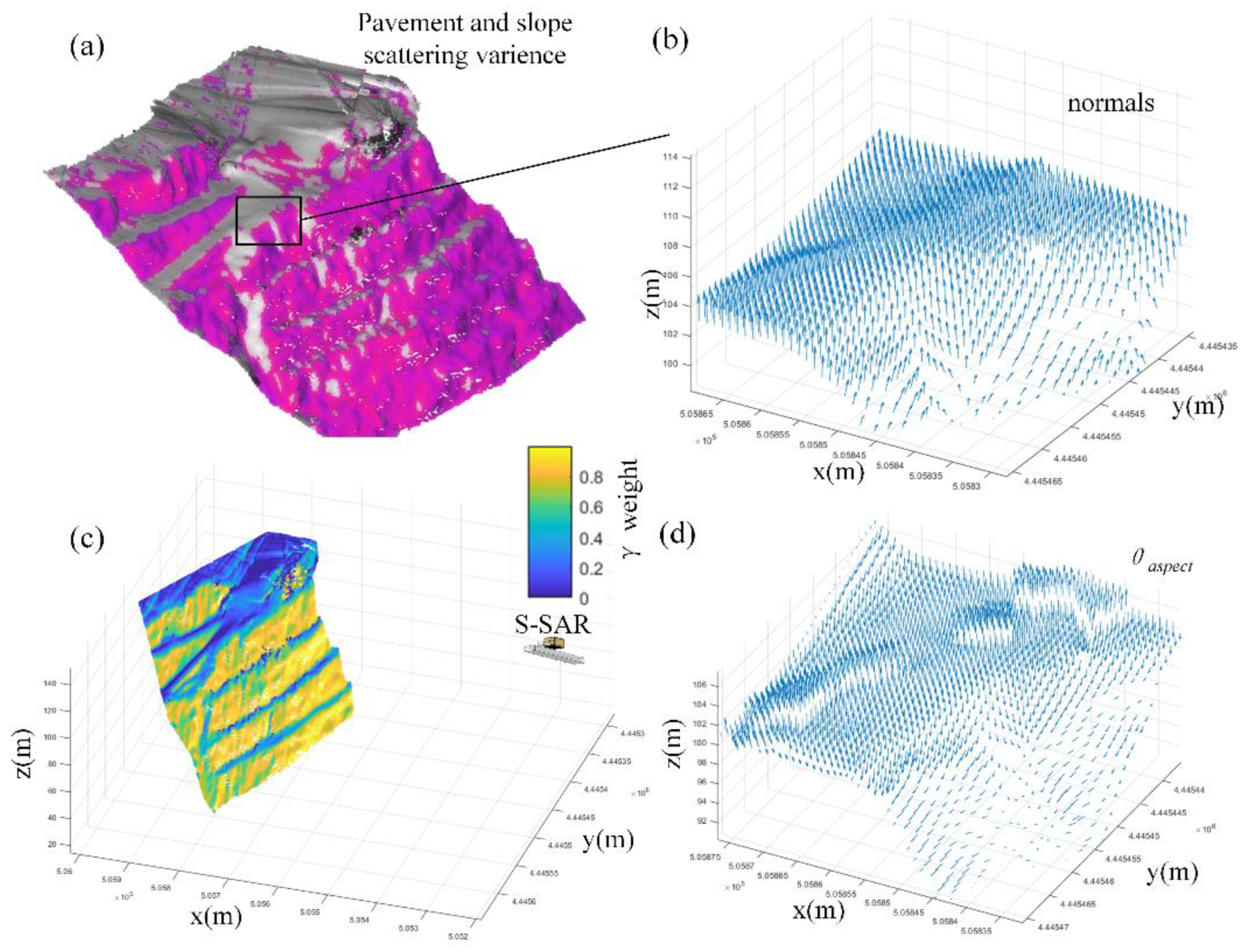
Target area real application: Firstly, the pavement and slope scattering variance can be extracted by the S-SAR microwave incident angle and is colored as shown in
Figure 11a. The bad incident areas have no color. The example figure of normal and calculated
is shown in
Figure 11b,d. The
shows that the sub-area would most probably move towards a given direction when affected by gravitation. However, when they are affected by other kinds of outside forces, the model should couple with the force analysis. Since the target area is a permanent slope which is only fluctuated by daily mining explosion, it can be treated as deforms along
vector. The weight
variance is shown in
Figure 11c. The areas with bad incident angles are shown as deep blue and brighter yellow areas are areas with good incident angles. As the road surface height went lower, the incident situation got better. The dark color of each road edge is the soil retaining wall which is to protect trucks from falling. The wall area weights also vary by incident angle changes. The nearest-neighbor mapping result and paper method result is as shown in
Figure 12.
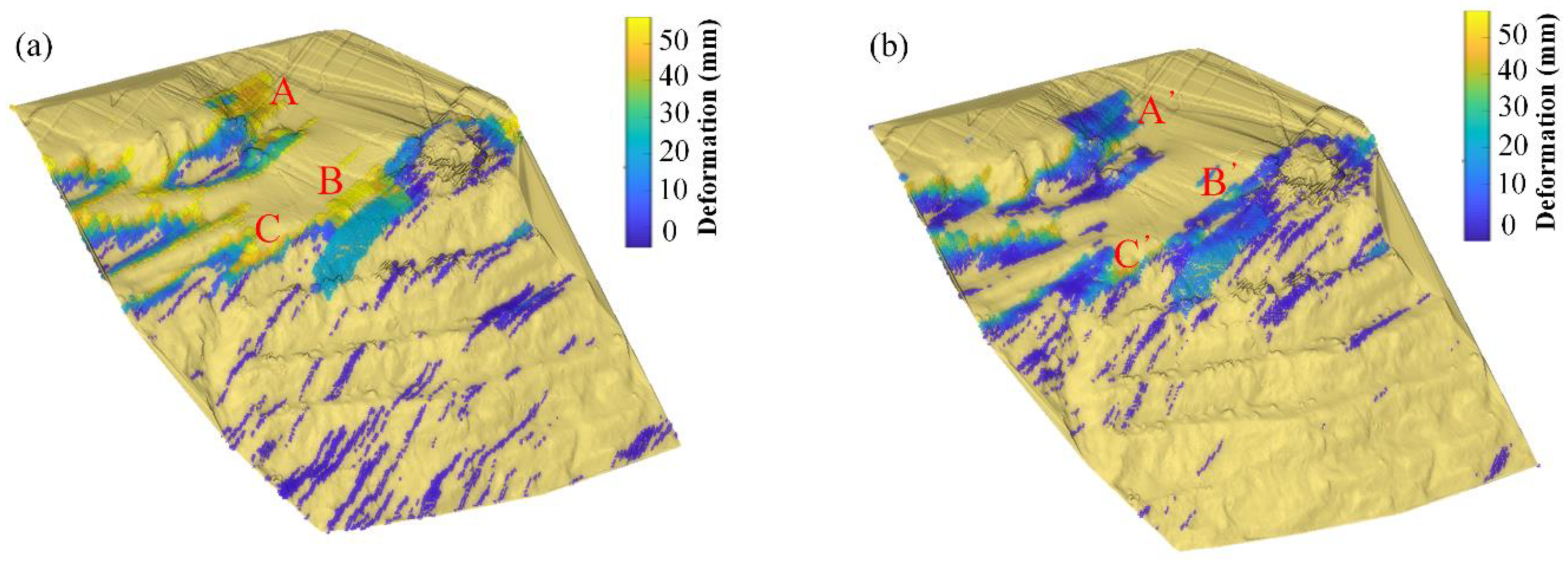
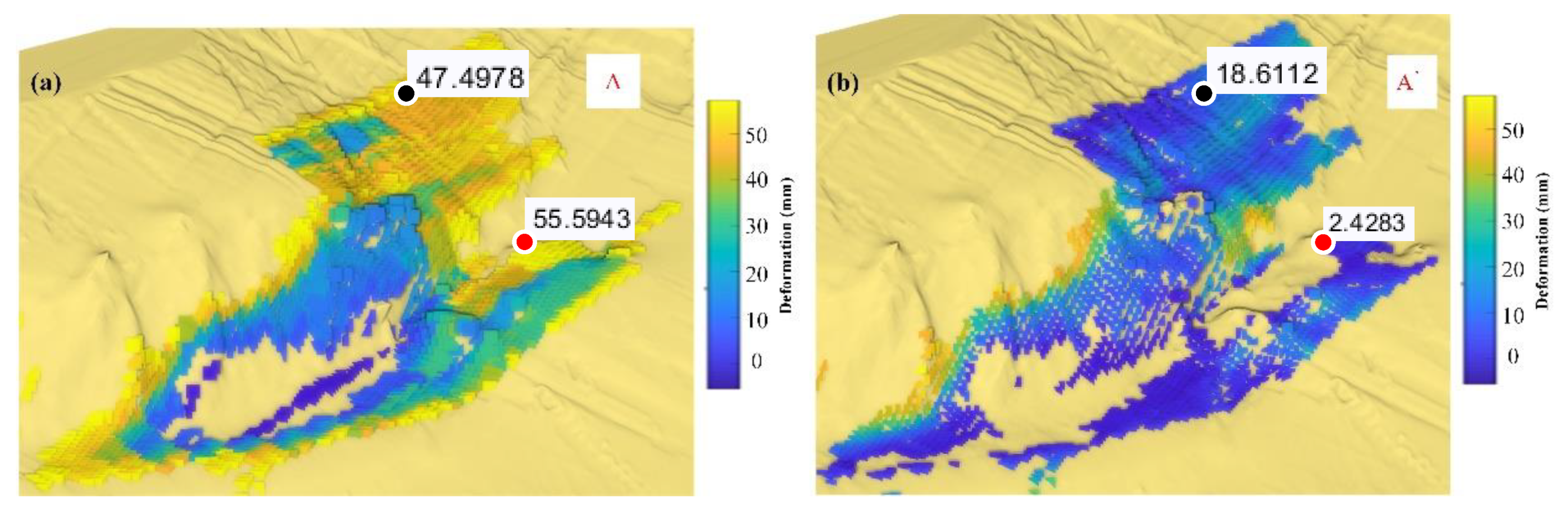
Three sub-areas A, A’, B, B’, C. C’ were selected, corresponding to the simulated step model sub-areas. Area A is as shown in
Figure 13a, the bright yellow boundary shows a great deformation, with the highest reach near 56 mm, which is quite large. The situation is quite similar to the controlled field test from in our previous work [
1], which are abnormal boundaries caused by the persistent scattering points that affect the neighborhood area. The area itself is not in a good coherence situation and the phase error is significant. Then, the deformation extracted in these boundary areas is also abnormal. In the A’ area, as is shown in
Figure 13b, the situation is relieved, especially for the pavement areas: For the red point, from 55.5943 mm to 2.4283 mm; for the black point from 47.4978 mm to 18.6112 mm. For the slope area, the real deformation still exists, a geologist can introduce their analysis method for further destruction deduction.
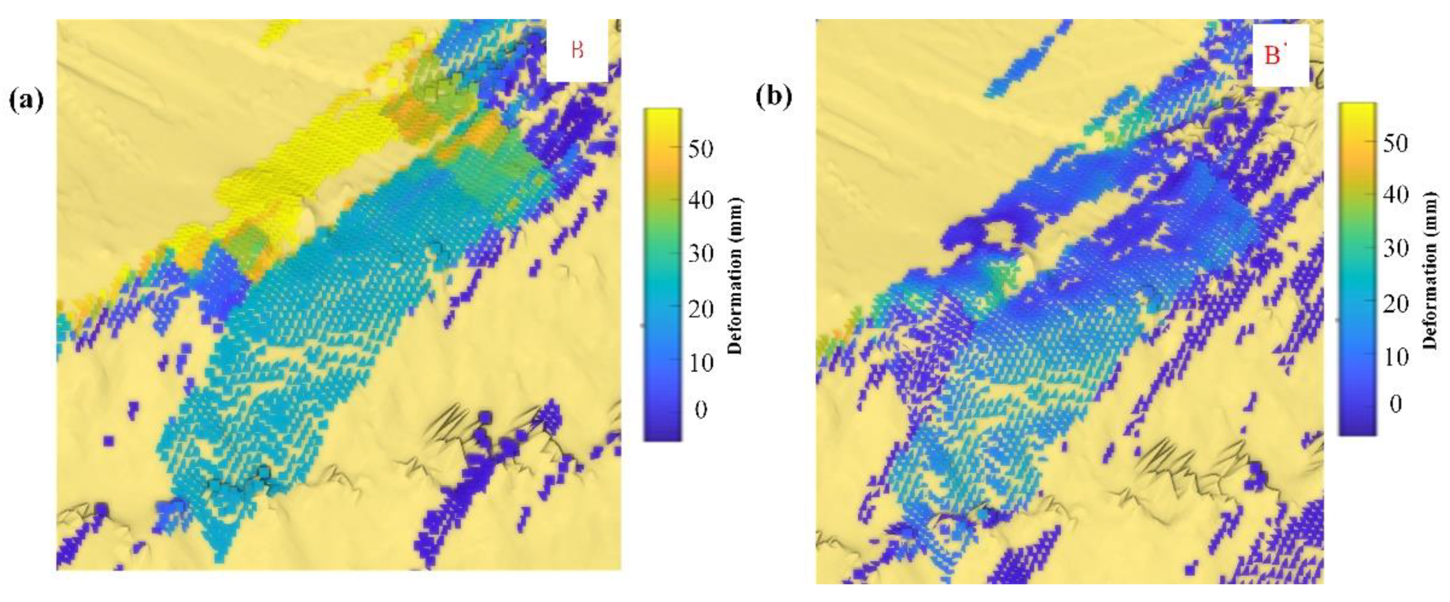
GB-InSAR monitoring is flexible, and monitoring geometry should be well designed to balance between layover distortion and shadow. The local incident angle and K-nearest neighbor patches aspect angle in the geometric and scattering model may help the layover distortion analysis (the case is shown in
Figure 14). The layover distortion would mostly happen when the SAR beam incident angle is near perpendicular. The area B and B’ show the same radar spatial resolution element. The B area shows no difference when across the road and slope. The sub-area deforms about 20 mm during the experiment. However, for the paper method, the B’ showed a difference as the incident angle changes. The road and slope were differentiated, and the inside small geo-elements deform according to their local shape. The result would help small area (less < 200 m
2) slide analysis, which often happens in open-pit mines.
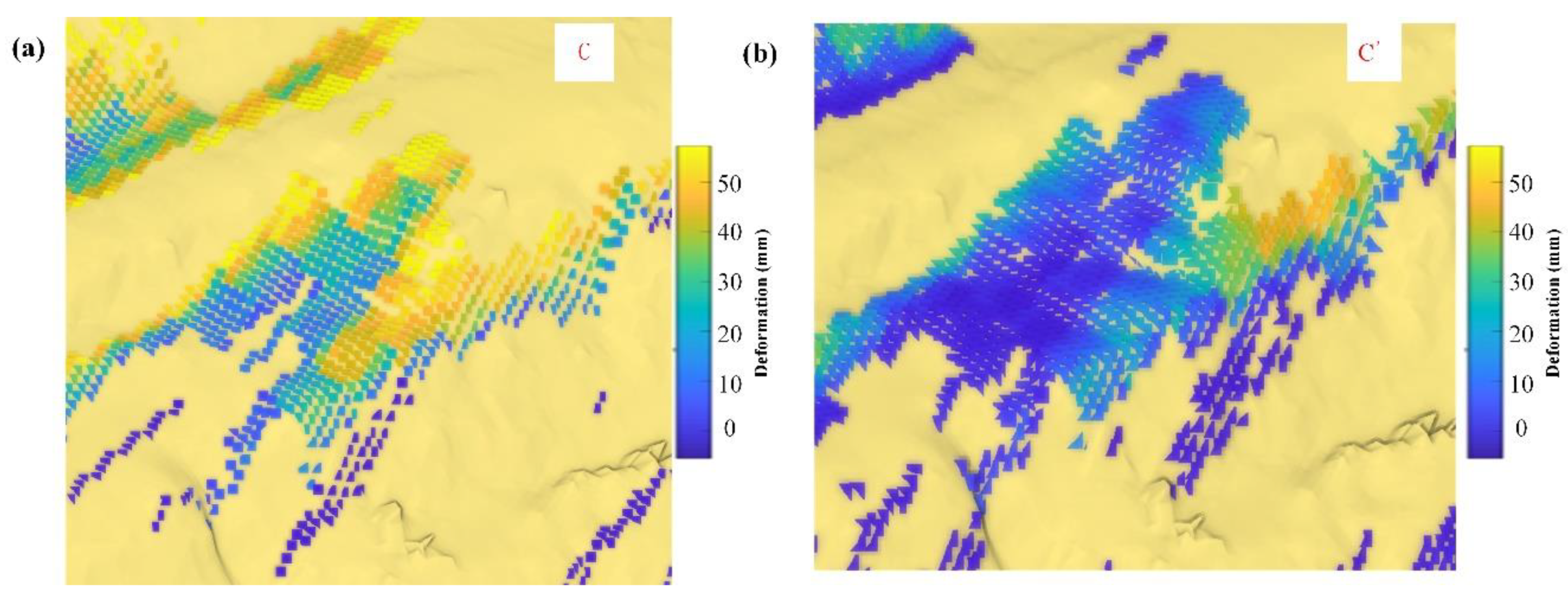
As shown in
Figure 15, the areas C and C’ show an area with an undulated surface. The case is quite similar to the road and slope crossing area. These areas are commonly seen in an open pit where roads go two directions, or the roads are a regional rotary; these are often unstable when trucks pass. The abnormal boundary was relieved by the proposed method in the paper. The nearest-neighbor method result is confused by abnormal deformation and the real deformed area is concealed.
5. Discussion
This section concentrates on the following issues:
In a strict sense, the weight calculated based on Equation (12) in the paper may not conform to the scattering differences of local areas in any natural scene. However, it is widely used in SAR image simulation. It comes from the hypothesis that the surface is a collection of “small spherical” scatterers. Some scattering model is simulated based on
function and a lot of researchers adopt the
function to simulate the scattering difference. In addition, if possible, we need to design our own compromise function to accommodate the local geological condition. The factor will affect deformation mapping. For example, the result in
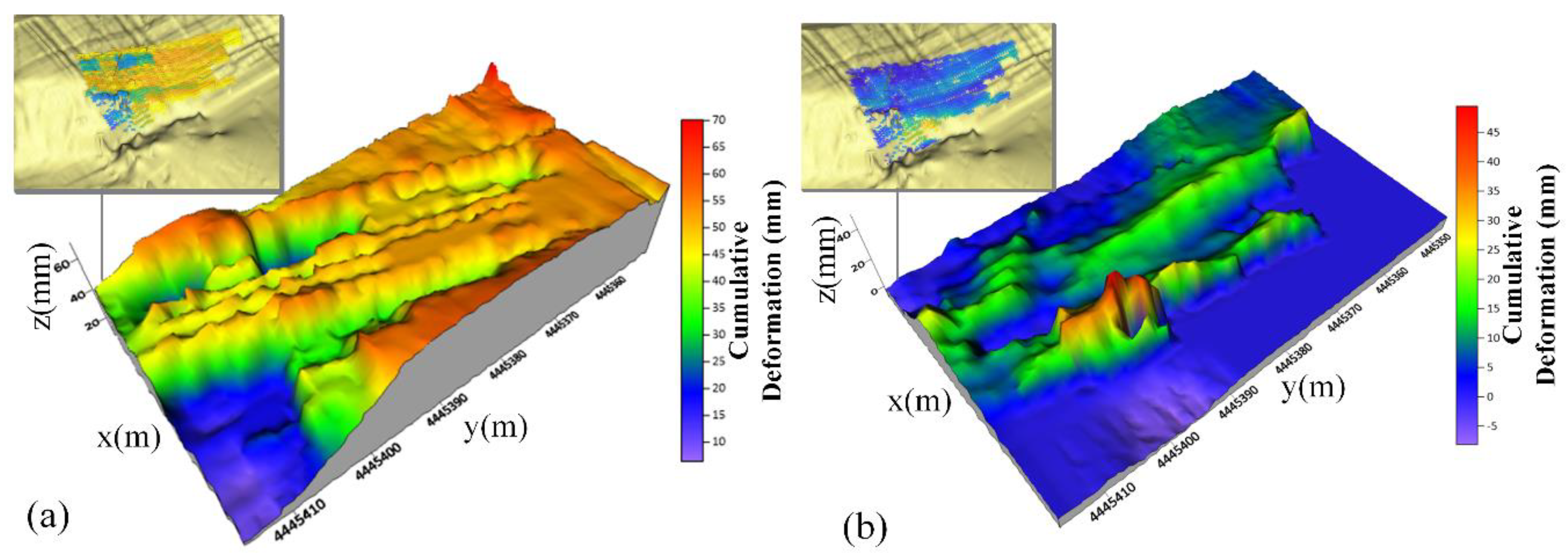
Figure 13 shows sudden changes from 40–50 mm to 20–30 mm. The situation may confuse us if the mapping result is correct or near the real deformation.
Figure 16a,b is the one radar pixel interpolated deformation surf plot of A and A’ (
Figure 13). The figure would help to understand the influences when using a geometric-scattering model.
According to
Figure 16, the following understanding can be concluded.
The GB-InSAR image pixel contains several targets. Due to the limited spatial resolution, these targets can be equivalent to one vital “scattering target”. The terrain point cloud model spatial resolution is higher than radar. The local area with a good incident angle in the radar pixel plays a major role in forming "sub-targets", and the shape variables are distributed on these distributed sub-targets. In this study, the deformation on the road surface is not eliminated, and their deformation is concentrated on the distributed sub-targets with good incident angles on the road surface.
If the precise deformation in the radar pixel is known through the ground control points or global navigation satellite system (GNSS) and other high time resolution measuring instruments, a more accurate model of mapping can be established. The optimizing objective function the least square solution of the temporal sequence deformation of each sub-target and the deformation function of the radar pixel.
From the perspective of geotechnical application, the difference between slope and road surface is highlighted, and the instability can be analyzed from a macroscopic perspective. Moreover, the model proposed in this paper can be integrated with the existing classical methods, rather than abandoning the previous methods. Fusion analysis is not the focus of this paper, and it will be further studied in the future.

 ,
, 


