1. Introduction
Signal processing is one of the most studied domains in the last decades. In the practical cases, most signals are not stationary and they are time dependent. Since non-stationary is a non-property, i.e there is no universal analysis tools in this case and we have to do the treatments separately for each case. In the late of 1950s, W.R. Bennett (1958) in [
1], saw that there is a type of non-stationary signals that have specific characteristics like hidden periodicity in their structures. Based on these characteristics, he introduced a new concept as an extension of the stationarity or as a special case of the non-stationarity which is “cyclo-stationarity”. Then, in the 80s, this concept was taken up by Prof. William A. Gardner with several applications in the telecommunication field [
2,
3].
In the last years, the cyclo-stationary tools played a pivotal part in the signal processing domain. It helped to improve monitoring, diagnosis and characterisation of systems in the rotating machine and telecommunication fields. Very recently several publications discuss the use of cyclostationarity in different technological fields [
4,
5]. In this paper we will be using these cyclostationary tools for the first time for turbulent machines. S.Tardu discussed in [
6] the implications of the cyclostationarity for the characterisation of turbulent flow, and the link between turbulent unsteady flow with imposed periodicity and cyclostationary process.
The aim of this paper is to contribute in the realisation of a software sensor that detects the fluid flow coming from a turbulent machine, than study this signal by the signal processing tools to model it. In each flow system we have a noisy part, and there are some works on removing this noise [
7,
8]. The original part in our paper is the using of the cyclo-stationary methods and the audio signals with the flow systems.
In fact to design an active control that eliminates the sound perturbation, it is important to analyse the mathematical and physical properties of the measured sound signal. On the other hand, in an industrial application, the noise disturbance have to be measured in real time. The entire device: acquisition of the sound signal and signal processing in real time to extract the useful information, constitutes a software sensor. The work presented in this paper deals with the analysis of the mathematical properties of the signal. Thus, a link can be made between the physical meaning of the sound signal and the useful part of the signal.
Hence, based on these methods, we can find the noisy frequencies, when each frequency has a physical realisation, then we can improve or eliminate the source of noise.
For a good treatment of the signals, we have to study the signal characteristics. We already know that flow systems aren’t stationary, that’s why we chose moving to the non-stationary tools and more precisely the cyclo-stationary ones. The comparison of our results by those of Jana HAMDI in [
9] and Sofiane Maiz in [
10] gives interesting results and made it possible to model these signals more clearly.
Section 2 presents some definitions, properties and extensions of the cyclo-stationary.
2. Cyclo-stationary: Definitions, Properties and Extensions
As a definition of the cyclo-stationary signal , it is a signal that has a hidden periodicity in its structure. We can distinguish different orders of cyclo-stationarity.
The first order cyclo-stationarity is when a signal’s mean (moment of order 1) is periodic in time. i.e.,
when T is the “cyclic period”.
The auto-correlation function (moment of order 2) is the dependence measurement between two different instants
and
(or
t and
). It is noted by
(or
) as the following:
or,
When
is equal to
. A signal who its auto-correlation function (moment of order 2) is periodic in time, it is called a second order cyclo-stationary signal. i.e.,
In a more general way, we can say that a signal is cyclo-stationary of order “n”, when its moment of order “n” is periodic.
When we have first order cyclo-stationary and second order cyclo-stationary in the same time, it results the “Wide-sense cyclo-stationary”.
There are some extensions for the cyclo-stationarity cited by J.Antoni in [
11] like “Pure and Impure cyclo-stationarity”, “poly-cyclostationarity” and “quasi-cyclostationary”, and others cited in [
12,
13] by F.Bonnardot like “Semi-cyclostationarity” and “Fuzzy Cyclostationarity”.
The most recent branch of cyclostationarity is the “cyclo-non-stationarity” that is introduced in 2013 by J. Antoni in [
14], and it cited as a solution of the “wide-speed variation” and the “run-up” problems.
Normally, when we study the cyclostationarity, we have to show our signal in the frequency domain. Hence, the calculation of the power spectral density (PSD) is very important. There are two ways to calculate the PSD. For the first method, the first step is applying the Fourier transform to the auto-correlation function compared to
. We obtain then the instantaneous spectrum or “Wigner-Ville spectrum”
. The second step is given by applying the Fourier series to this instantaneous spectrum compared to
t to obtain the “cyclic power spectra”
or the PSD
when
is the cyclic frequencies and
[
10,
15,
16]. If
is stationary then we apply this method with
.
The second way has also two steps. The first one is to calculate the “cyclic auto-correlation function”
by applying the Fourier series compared to
t. then we apply the Fourier transform compared to
as the second step to obtain
or
[
16].
Another function also very important in our work is the “cyclic spectral coherence” (SCoh). A cyclostationary signal has correlations in its spectral components spaced apart by the cyclic frequencies
. The strength of these correlations is measured by the cyclic coherence function [
16]. It is defined as
with
.
In the
Section 5 we will be using the power spectral density PSD and the cyclic spectral coherence function SCoh to model our signal and detect the noisy frequencies. To calculate these two functions we used the methods presented by J. Antoni in [
16].
5. Experimental Results
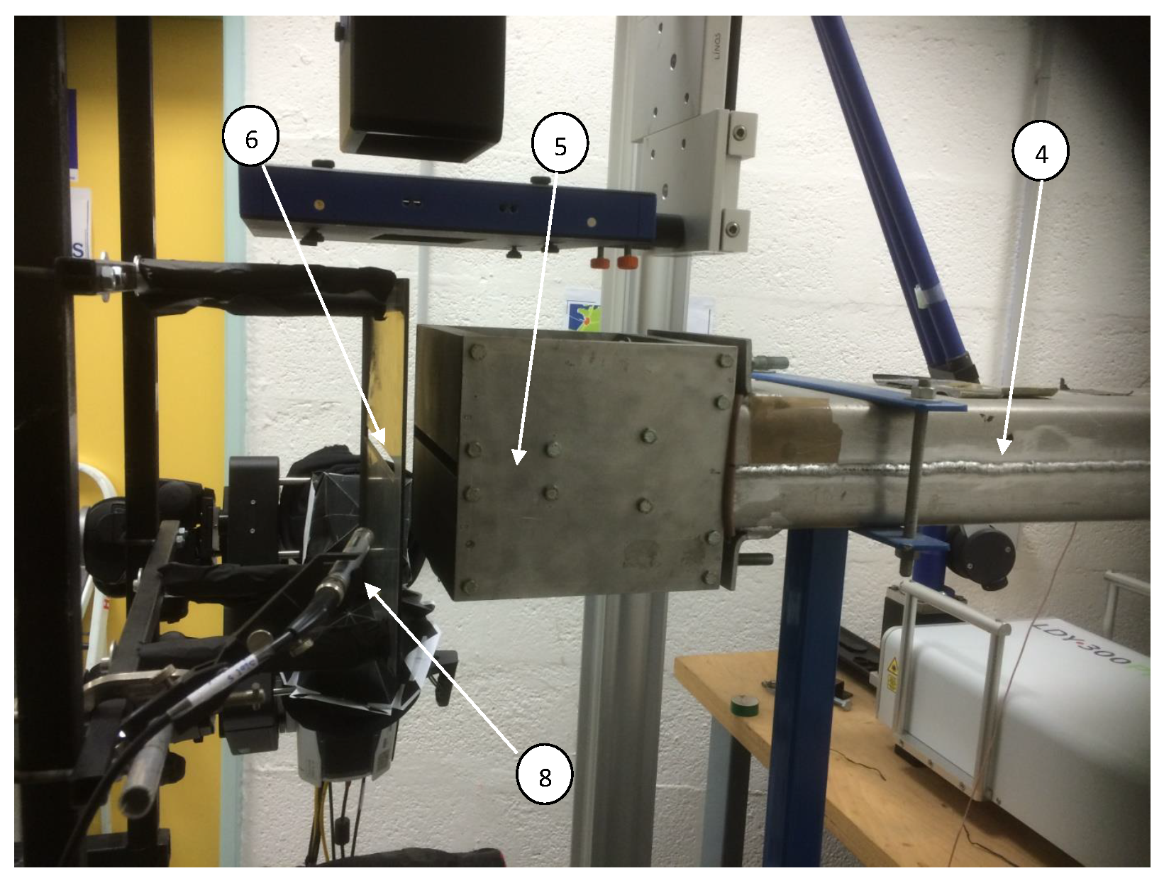
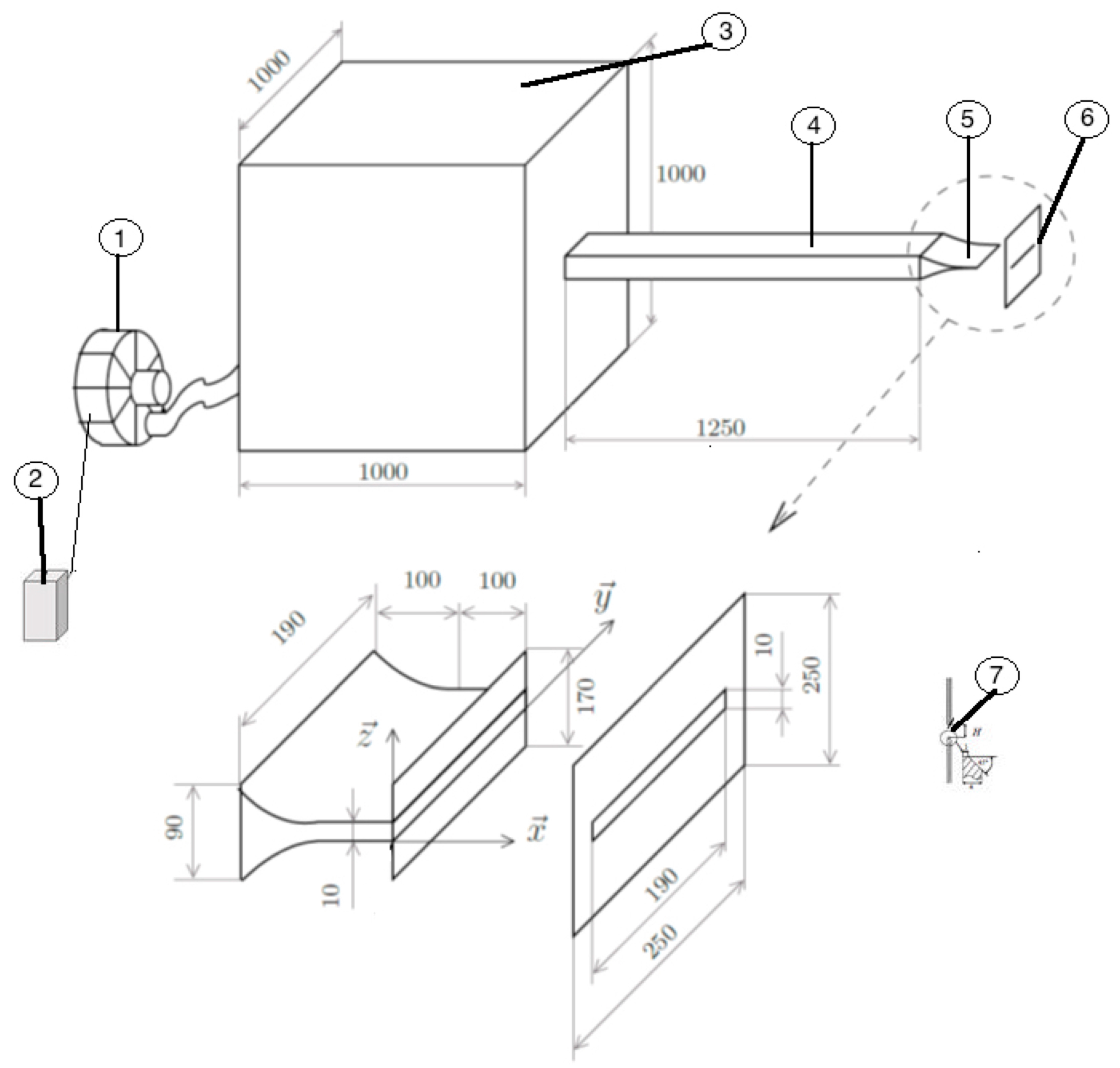
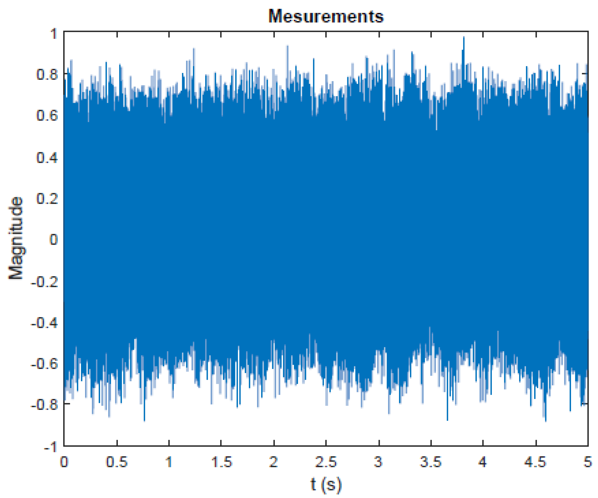
For the processing, we take the recordings obtained from the microphone 8. The
Figure 5 plots the measurements in a sampling frequency equal to 10 kHz for a duration of 50,000 samples. With a frequency resolution of
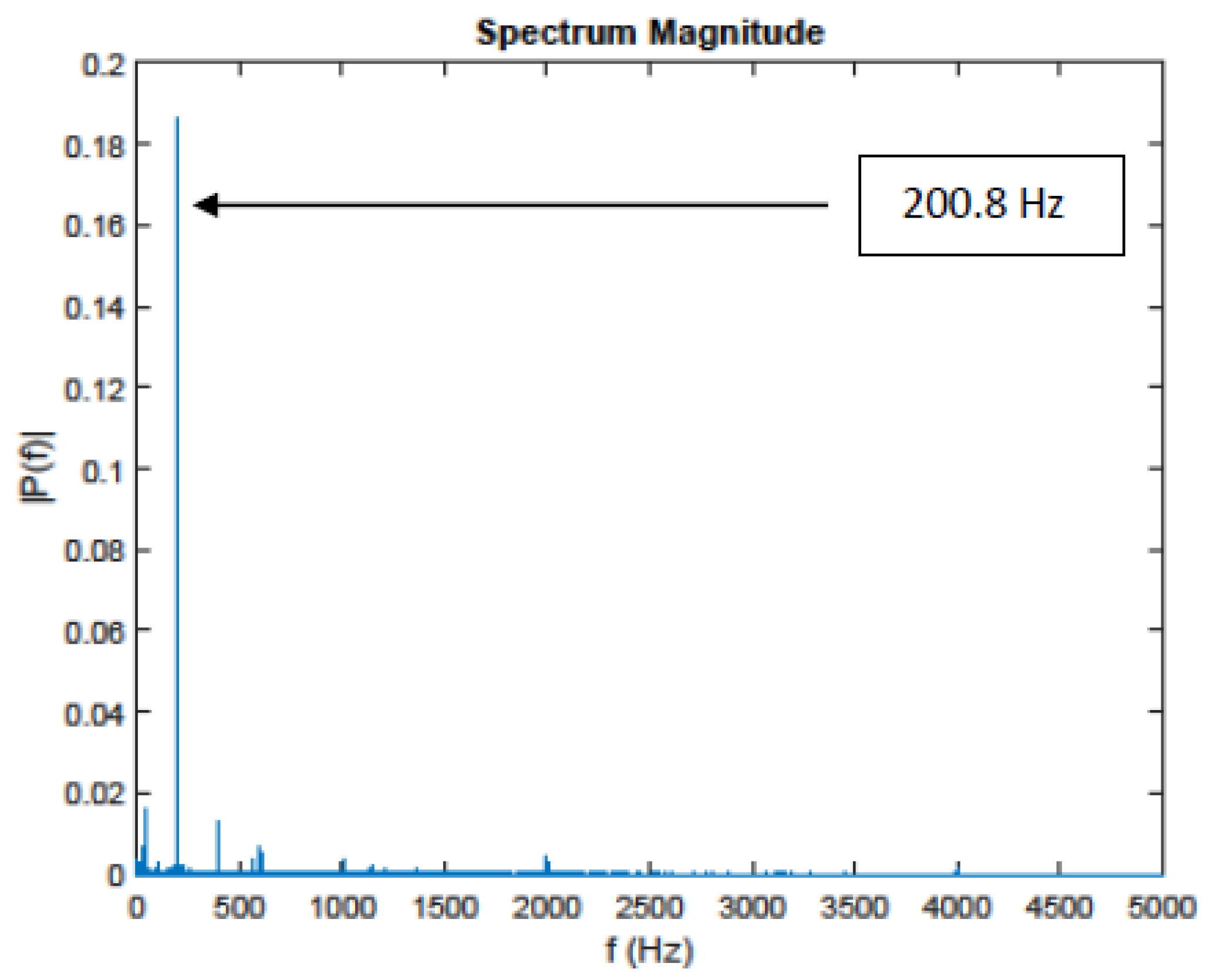
= 0.2 Hz, the use of FFT will perform the spectrum of the signal. This spectrum is plotted in the
Figure 6.
Every frequency present in the spectrum during the use of the FFT calculation must be stationary. The use of FFT, in the case of the non-stationary signal, provides a result that is not entirely accurate. For our case, over the time horizon of 5 s, the characteristic frequency moves. The value of 200.8 Hz corresponds to a kind of “average”. The proposed method improves its characterization by specifying its properties. This characterization is important in order to then follow the evolution of the characteristic frequency in real time. Hence, for the presence of the non-stationary part of our signal, we chose to apply the cyclo-stationary methods, i.e.,to calculate the cyclic spectral density and the cyclic spectral coherence of the measurements.
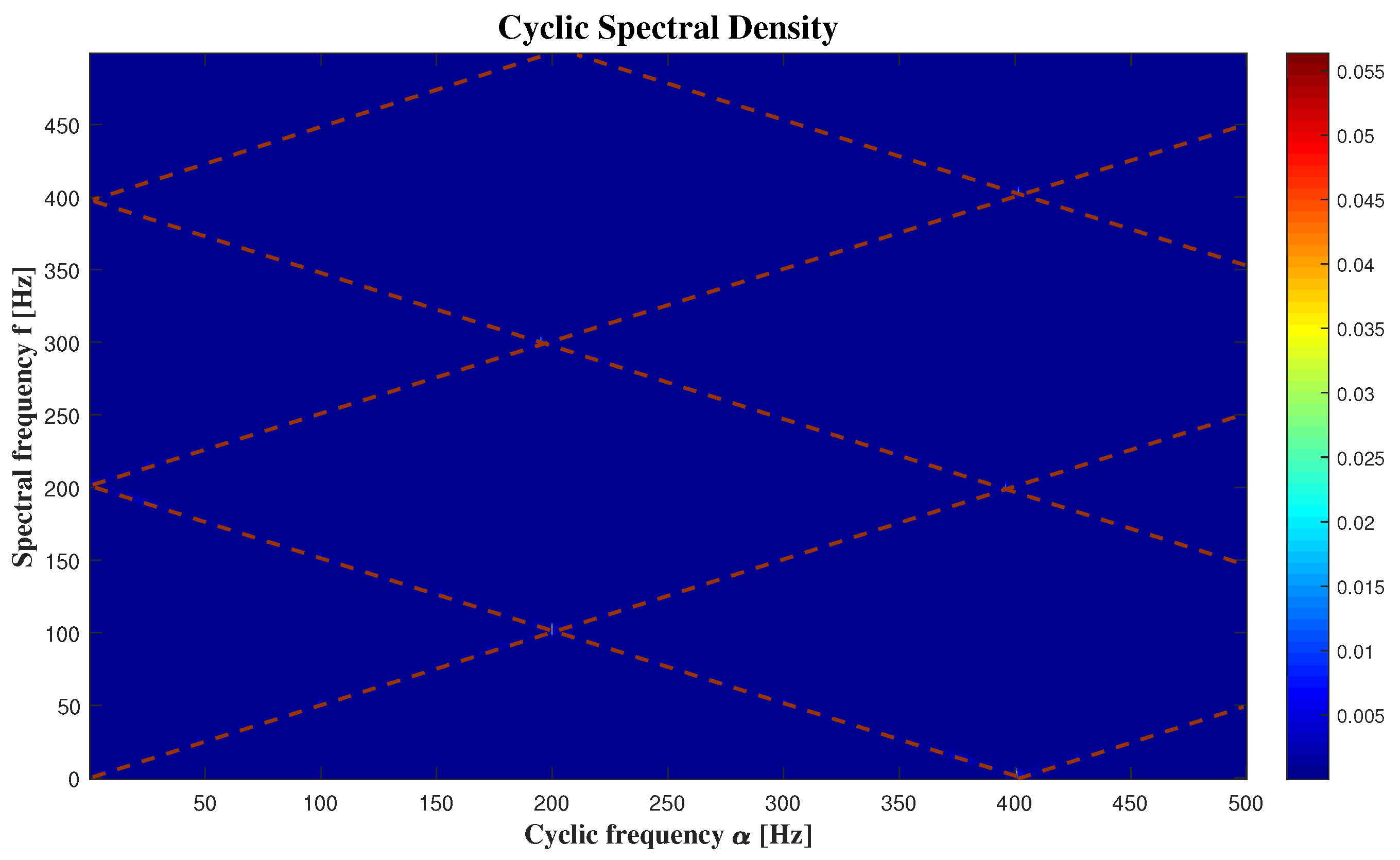
The
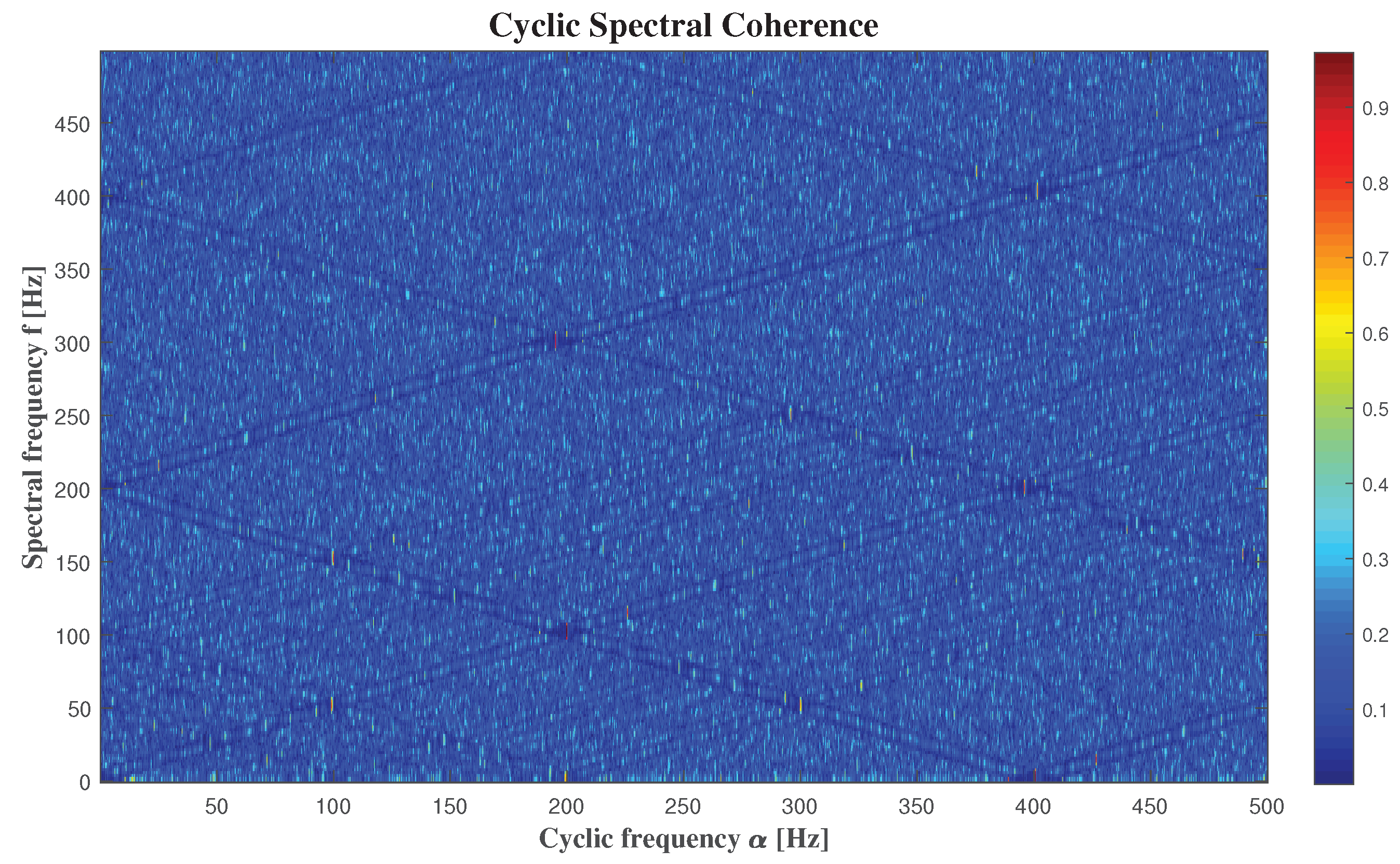
Figure 7 presents the Welch’s estimate of the (cross) cyclic power spectrum of the signal coming from microphone 8, and the
Figure 8 displays Welch’s estimate of the cyclic spectral coherence of the same signal. We obtain by the two
Figure 7 and
Figure 8, that the results are the same by using these two methods, but it’s more detailed with the cyclic spectral coherence. That’s why the using of cyclic power spectrum is not enough.
Maiz Sofiane presents in [
10] the theoretical relations between the cyclic frequency “
” and the delay parameter “
”, then he classifies the types of signals based on these relations and the model in Equation (
9).
Based on [
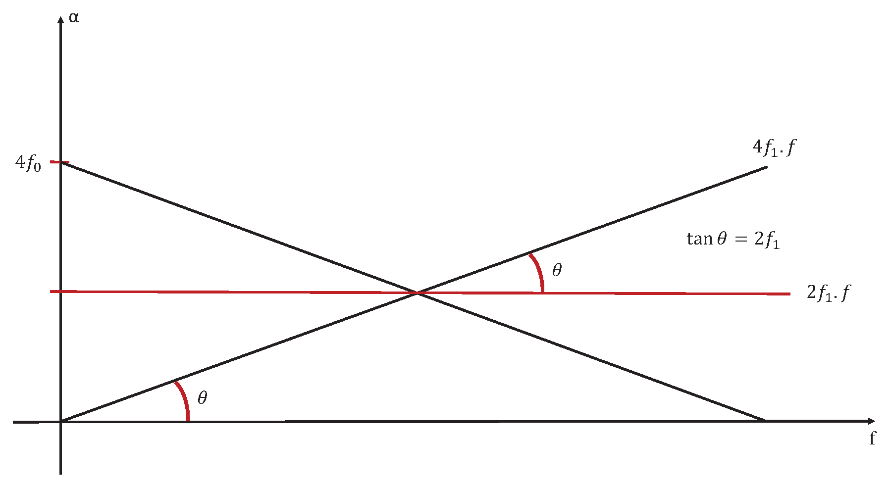
10], we can represent the case of signal
, when it’s a stationary signal like in
Figure 9, or a cyclostationary one as in
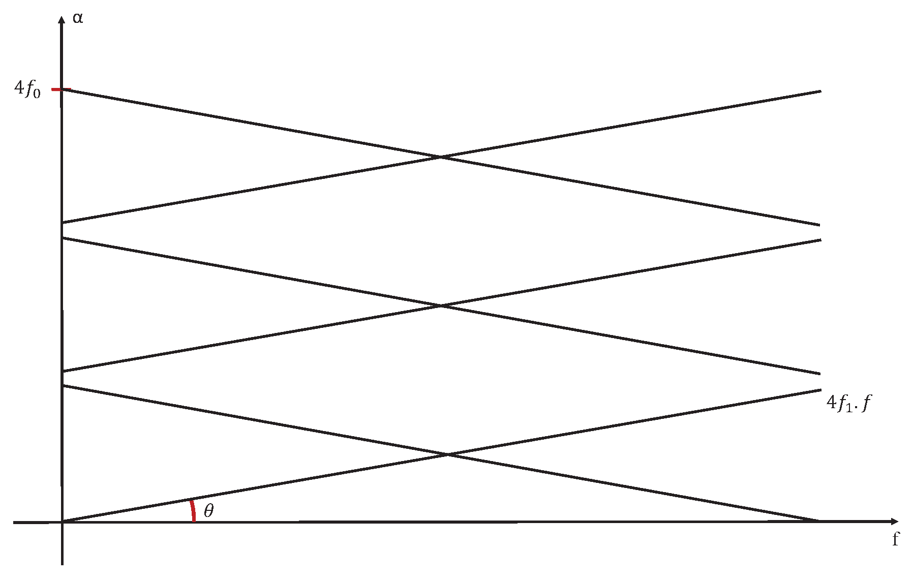
Figure 10.
However, in our paper, we chose to set the relation between the cyclic frequency “” and the spectral frequency “f” apart from the delay “”, when “f” is the spectral representation of “” in the frequency domain.
We can clearly see that the relation between “
” and “
f” presented in
Figure 7 and
Figure 8 is represented by
Figure 10. Then we can consider that we have a generalised cyclostationary signal
equal to
and our model is equal to:
With
,
Hz,
Hz,
Hz.
When we compare our model to the one in [
9], the authors said that the model form is sinusoidal, like ours, which is a good indication of eddies passage.
We can also detect the noisy parts of the audio signals in
Figure 7 and
Figure 8 by looking at where the frequencies are giving us high intensities. Based on these figures, it is clear that the frequency that gives us the high intensity in
Hz, is equal to
, and its harmonics. It is expected, because
is the responsible of the amplitude of our signal.
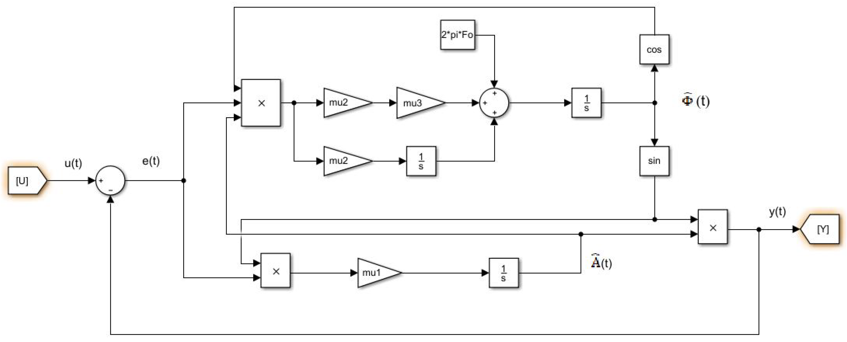
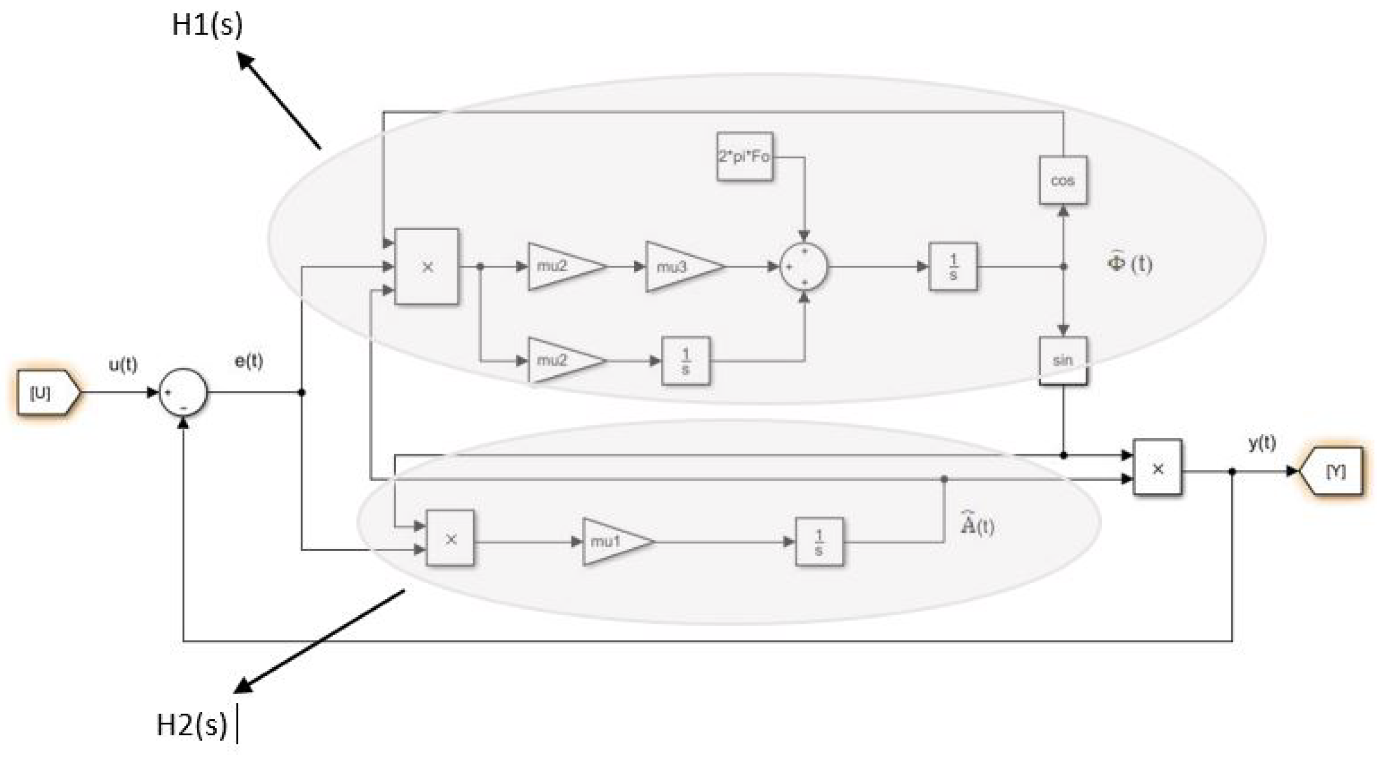
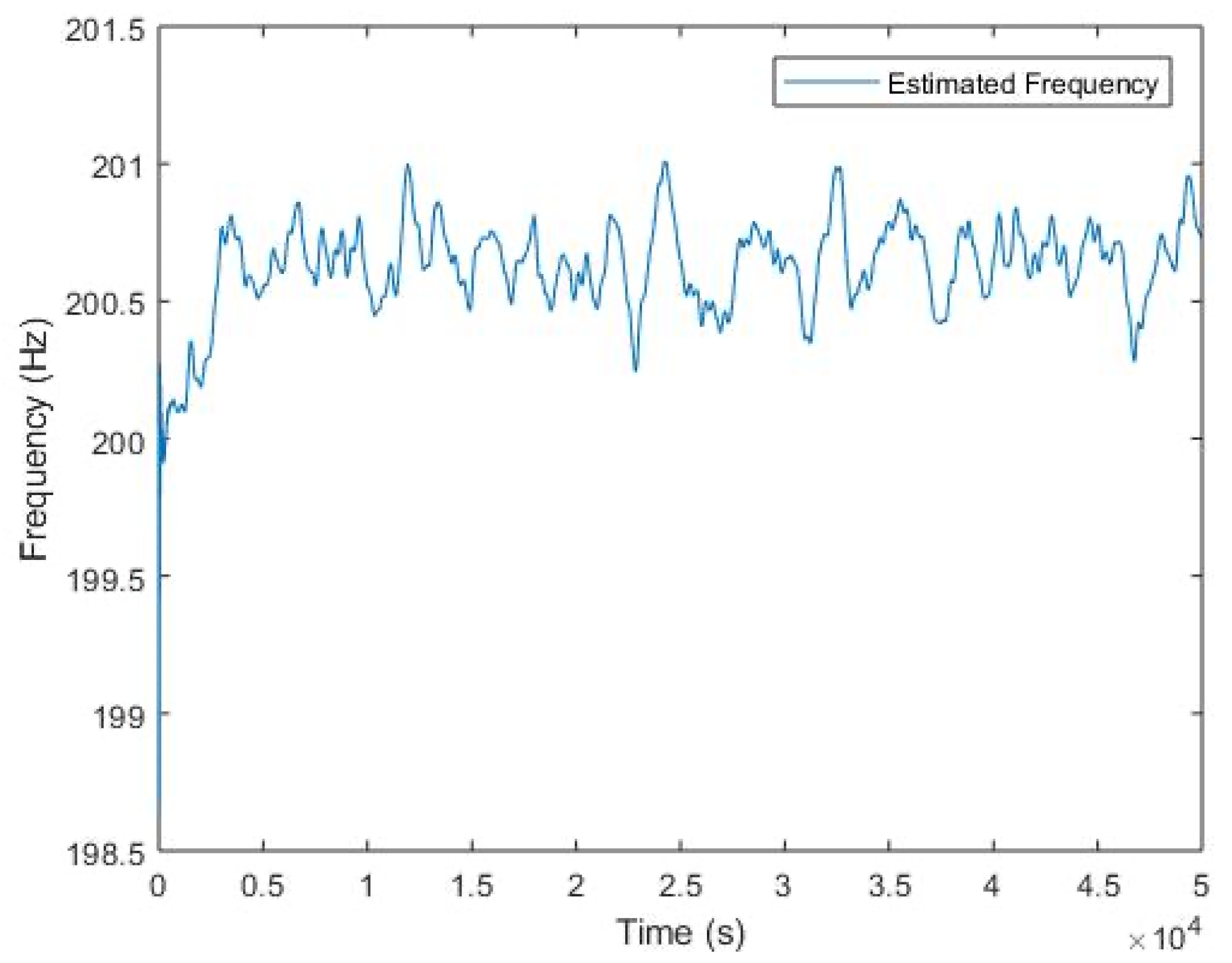
In a real time context, the algorithm presented in
Section 3.2 allows to extract the frequency
. The
Figure 11 presented the result obtained with real signal.
6. Conclusions and Discussion
This paper presents a software sensor development with signal processing tools to model the signals coming from a turbulent machine, and detect the noisy frequencies which are representing physical materials producing the noise. A first analysis based on the use of the FFT tool gives an overall idea of the characteristic frequency. However, this analysis is not sufficient, the physical phenomenon is not stationary. Before proposing a “real-time” monitoring of the characteristic frequency, we propose to demonstrate a property of generalized cyclostationarity of the signal. The use of cyclostationary methods is recommended in this case because of the cyclic airflow created by the turbulent machine. It is thus possible to characterise the experimental setup from the point of view of noise pollution in a precise and dynamic way.
These results have similarity with those in [
9] and integration by using software sensor and cyclostationarity tools which are easy to apply and gives good treatment and modelling. We can also use this software sensor to diagnose the machine apart from modelling and noise detection, by other words, for fault detection and perhaps prognosis because of the cyclostationary using.
The algorithm presented in
Section 3.2 allows realization of a “real-time” experiential device. To follow a non-stationary frequency that changes around 200 Hz, the sampling frequency is not a technological problem. This software sensor enables tracking a particular frequency dynamically and developing a control law to attenuate the noise nuisance in future work.

 ,
, 


