Abstract
The recent Wi-Fi HaLow technology focuses on adopting Wi-Fi for the needs of the Internet of Things. A key feature of Wi-Fi HaLow is the Restricted Access Window (RAW) mechanism that allows an access point to divide the sensors into groups and to assign each group to an exclusively reserved time interval where only the stations of a particular group can transmit. In this work, we study how to optimally configure RAW in a scenario with a high number of energy harvesting sensor devices. For such a scenario, we consider a problem of device grouping and develop a model of data transmission, which takes into account the peculiarities of channel access and the fact that the devices can run out of energy within the allocated intervals. We show how to use the developed model in order to determine the optimal duration of RAW intervals and the optimal number of groups that provide the required probability of data delivery and minimize the amount of consumed channel resources. The numerical results show that the optimal RAW configuration can reduce the amount of consumed channel resources by almost 50%.
1. Introduction
The concept of the Internet of Things (IoT) [1] with its tremendous number of interconnected autonomous devices has become very attractive for device vendors, mobile operators, and their customers [2]. In addition to whipping up the telecommunication market, IoT brings new services and applications, which will revolutionize our life. From the technical point of view, it is evident that the easiest way to provide Internet access for the swarm of devices is using wireless communications. At the same time, it is not clear how to do it the most efficiently.
Another challenge is the energy consumption. Since it may be difficult, if even possible, to wire thousands of devices to an electric grid, autonomous devices are typically battery-supplied and/or harvest solar, wind, or other kinds of green energy. Using green energy may be especially fruitful in rural deployments, e.g., for agriculture monitoring. However, energy harvesting still needs energy storage. Unfortunately, from both technical and ecological points of view, the usage of traditional accumulators by autonomous devices is limited. First, their efficiency degrades with every recharge cycle. Second, they typically contain much mercury, cadmium, lead, or other dangerous poisonous materials. That is why, in many scenarios, autonomous devices have rather small energy accumulators or even capacitors [3,4,5].
Both low energy consumption and a high number of devices occasionally transmitting short messages are the main challenges for IoT networking protocol developers. To handle them, many international organizations and standardization bodies are currently developing new telecommunication standards or adapt existing communication technologies to IoT. Thus, LoRa can be used together with vibrational energy harvesters for bridge monitoring [6] or with RF energy harvesters for health monitoring in construction [7]. Another example of the successful application of telecommunication technologies with energy harvesting is the usage of Bluetooth Low Energy (BLE) with ambient light energy harvester [8] or RF energy harvesters [9] in Smart Building scenarios, e.g., to track the room occupancy.
LoRa and BLE have been designed for long and short range communications, respectively, and provide rather low data rates. The intermediate niche can be occupied by the Wi-Fi Halow technology. It is based on the IEEE 802.11ah [10] amendment to the Wi-Fi standard, and is designed to make Wi-Fi suitable for communication of swarms of autonomous devices [11]. Similarly to LoRa, it operates in sub 1 GHz frequencies, but uses wider channels (from 1 MHz to 16 MHz) and can provide much higher data rates (up to ≈347 Mbps). As a result, it can be used in sensing scenarios, such as residential scenarios (smart meters, elderly care) or environmental and agricultural monitoring with a transmission range of < 1km [11]. Such scenarios are a perfect match for energy harvesting batteryless sensors [8,9,12] to be used in conjunction with Wi-Fi HaLow. These sensors can harvest RF, thermal, solar, or mechanical energy [13].
A key component of the 802.11ah amendment is the Restricted Access Window (RAW): a novel channel access method, which allows for reducing the number of stations (STAs) accessing the channel simultaneously and thus limits the contention for channel access between the STAs. The contention of a high number of STAs results in collisions. According to [14], collisions are the main source of energy losses in Wi-Fi networks.
RAW allows an Access Point (AP) to divide the STAs into several groups and assign each group to a time interval during which only this group can access the channel. Thus, RAW allows the AP to limit contention between energy limited STAs. In addition, it protects the transmission of these STAs from collisions with other STAs, e.g., offloading STAs connected to the same AP.
Offloading is the second important use case for IEEE 802.11ah thanks to the long transmission range and relatively high maximal throughput. It is a feasible and cheap way to meet the clients’ requirements on throughput and latency in cellular networks. In a big city, cell phone users are in Wi-Fi zones for 70% of their time, and 65% of mobile traffic can be offloaded [15]. An IEEE 802.11ah network can be used both for gathering data from energy-limited sensors and for serving the offloading STAs, and there is a trade-off between the channel resources allocated to each kind of STA. On the one hand, enough channel resources should be allocated (with RAW) to the energy-limited STAs so that they can deliver their data. On the other hand, it is necessary to leave as many channel resources to the offloading STAs as possible to avoid network underutilization.
The RAW mechanism has been extensively studied via simulation [16,17] and mathematical modeling [18,19,20,21,22,23,24,25,26,27,28,29]. In this paper, we focus on analytical approaches to estimate the network performance and note that most papers that analyze the efficiency of Wi-Fi networks with RAW incorrectly describe the data transmission with RAW. Most related works [18,19,20] consider saturated traffic which is not a typical IoT scenario, while those that consider non-saturated traffic [21,22,23,24,25,26] mostly neglect the fact that the data transmission process within the allocated time intervals is non-stationary, i.e., the probabilities of transmission attempt and collision change with time. At the same time, the papers which correctly model the non-stationary data transmission process [27,28,29] do not consider the possibility of STAs running out of energy during the transmission process, but such an event is quite likely and important in IoT scenarios due to the following reasons. Firstly, the packet losses in wireless sensor networks can be caused not only by noise in the channel and contention for channel access but also by the depletion of STA energy. Secondly, when STAs run out of energy, they stop contention for channel access, and thus, the conditions for the other STAs are improved, which also affects the packet loss rate. Thus, it is important to consider the amount of energy available for the STAs while studying the data transmission solutions for wireless sensor networks.
The core contribution of this paper is the performance evaluation of the channel access method introduced in the 802.11ah amendment in networks with energy-harvesting devices. For that, we significantly extend our approach previously developed in [27,28] to model RAW behavior. In contrast to [27,28], in this paper, we consider a more complex scenario when we develop our mathematical model.
First, the STAs are energy harvesting and are supplied by a limited source of energy, so, during the transmission within the RAW slot, an STA can stop contending for the channel because of the depletion of the energy. This factor is important for two reasons. On the one hand, an STA that does not have enough energy fails to deliver its traffic during the RAW slot. On the other hand, when other STAs stop contending for the channel, the probability of successful transmission for the considered STA increases.
Second, the transmission attempts can fail because of collisions and the random noise in the channel, which is new.
With the developed mathematical model and simulation, we find non-obvious effects, which we describe and explain in the paper. Finally, we show how to use the model to find an optimal RAW configuration, i.e., such RAW parameters that minimize channel time consumption by the energy-harvesting devices and, at the same time, guarantee the delivery of the data with the required probability. We also show that the usage of models that does not take into account the limited sensor’s energy and the parameters of random noise in the channel can lead to an incorrect choice of RAW parameters, which cannot provide the required probability of data delivery.
The rest of the paper is organized as follows. In Section 2, we describe the studied scenario in more detail and state the problem solved in the paper. Section 3 reviews the papers related to the subject of wireless energy-limited device networks, IEEE 802.11ah networks, and data transmission in Random Access Window. In Section 4, we design an analytical model to solve the stated problem. In Section 5, we present and discuss the numerical results obtained with the model. Section 6 summarizes the main results of the study.
2. Problem Statement
2.1. Channel Access Method
The core idea of RAW is that an AP can select several STAs and allocate them a time interval called the RAW slot, during which only the selected STAs can transmit their packets while the other STAs are forbidden to access the channel. The AP can allocate a single RAW slot to a group of STAs or can establish a long-term periodic RAW slot allocation (so-called Periodic RAW or PRAW). With PRAW, the AP allocates to a group of STAs a series of equidistant time intervals of the same duration. In this article, we consider the PRAW approach since it introduces less overhead than repeating a single RAW slot allocation.
To access the channel during its RAW slot, the STA uses a native Wi-Fi enhanced distributed channel access (EDCA), which implements Carrier Sense Multiple Access with Collision Avoidance (CSMA/CA). In summary, it works as follows. At the beginning of the slot, the STA initializes a backoff counter with a random integer value equiprobably drawn from the interval , where is the minimal contention window (a configurable network parameter). If the channel is idle during time , the STA decrements the backoff counter. If the channel is busy, the STA freezes its backoff counter and waits until the medium becomes free. It unfreezes the backoff counter when the channel has been idle during the arbitration interframe space (). When the backoff counter reaches zero, the STA transmits its data frame, provided that the transmission, including the expected acknowledgment frame (ACK), ends before the termination of the RAW slot.
If a frame transmission fails because of the random noise or collisions, the ACK does not arrive. Thus, the STA considers the transmission attempt as unsuccessful and increments the retry counter r (initially set to zero). If the retry counter reaches the Retry Limit , the pending frame is dropped. Otherwise, the STA repeats the transmission attempt. For that, it equiprobably draws a new backoff value from doubled contention window , where
2.2. Scenario
Let us consider a network with an AP, many energy harvesting sensor STAs, and several offloading STAs. From time to time, energy-harvesting STAs generate some small portion of information and intend to transmit a packet with this information to the AP. The packet shall be delivered to the AP no later than after it has been generated. Otherwise, it becomes outdated and is discarded by the STA. Additionally, the ratio of delivered packets shall not be less than . To simplify the further analysis, we assume that all packets have the same size.
The AP divides energy-harvesting STAs into several groups and assigns a periodic series of RAW slots to each group. The energy-harvesting STAs transmit their packets only in their own RAW slots. The offloading STAs are allowed to transmit only outside the allocated RAW intervals, as shown in Figure 1.
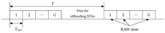
Figure 1.
The Periodic RAW scenario.
We consider that the STAs assigned to the same RAW slot are located in the transmission range of each other, i.e., they are not hidden from each other. Such an assumption is reasonable because IEEE 802.11ah provides several ways to avoid hidden STAs and improve performance. First, during the association process, the AP can determine the direction for each sensor STA and then group STAs with respect to their locations. Second, it can use the sectorization mechanism, which allows only those STAs to transmit that are located in a given sector [18,30].
Every STA generates a Poisson flow of packets, the intensity of which is much lower than and the period of RAW slots allocated to the STA. Having generated a packet, an energy-harvesting STA waits for its slot and tries to deliver the packet. A transmission attempt may fail because of the random noise in the channel or collisions. The STA’s transmission is damaged by noise with probability p.
If the transmission attempt is unsuccessful, the STA repeats it if the retry limit is not reached. As soon as the packet is successfully delivered, the STA switches off its radio interface to save energy.
The STAs are supplied by a capacitor or small accumulator and can slowly harvest the energy from the environment, e.g., using a solar cell, motion, or an RF energy harvester [31]. We assume that at the beginning of the RAW slot, the STA has a random amount Q of energy, which it has harvested since the last transmission attempt. When an STA listens to the channel or tries to transmit a frame, it consumes energy. As in [32,33,34], if the STA’s energy becomes less than the amount required to transmit a frame, the STA switches off its radio interface at least until the next RAW slot, even if its packet is not delivered. In addition, the STA switches off its radio at the end of the RAW slot.
Since this research is focused on the evaluation of channel access in Wi-Fi HaLow networks using RAW, we consider a simplified model of energy harvesting and, similarly to [32,34,35], assume that the amount of energy that the STA harvests since the last transmission attempt linearly depends on the elapsed time, i.e., we consider that the fluctuations related with the instability of the energy source, e.g., the variability of the solar flux caused by the clouds, are averaged over a sufficiently large period of time. In our scenario, it is justified by the assumption that the RAW period is much higher than the RAW slot duration. The average amount of of energy harvested by the STA within a RAW period is a variable parameter that characterizes the energy harvesting system, e.g., the solar cell area.
As the frame delay budget is , the period of RAW slots shall not be greater than . At the same time, the period of RAWs less than is also inefficient. To clarify this statement, let us consider a group of STAs that is granted a series of RAW slots. Let us fix the channel resource consumption defined as the time that the group is allowed to transmit and consider two cases. In the first case, RAW slots follow with period T, and their length is . In the second case, RAW slots follow with period and their length is , where . In the latter, STAs have less time for transmission, but the more important problem is that the contention windows the STAs had at the end of the RAWs are not kept. Therefore, they spend more time with small contention windows and hence high collision probability, wasting energy. For that reason, we consider only the scenario when the RAW period is .
For the described scenario, we state the problem to find out how to divide STAs into groups, and to determine the RAW slot duration for each group in such a way that the channel resource consumption by the STAs is minimized, but the restriction on minimal packet delivery ratio is met. To solve this problem, we develop a model of the described above process.
3. Related Papers
In the literature, many papers study various aspects of energy-efficient data transmission in wireless sensor networks. A group of studies consider abstract wireless sensor networks and derive general models of their operation using the Markov models [36], Energy Packet [37,38] abstraction, or the Brownian motion [39]. Another group of studies consider wireless sensor networks using different technologies, including the cellular networks [40,41] such as NB-IoT [42], low power wide area networks such as LoRaWAN [43,44], and wireless personal area networks such as ZigBee [45]. Finally, some papers evaluate the benefits of low-power wake-up radios added to existing technologies to reduce power consumption, e.g., see [46,47] for Wi-Fi and 5G networks. However, since this paper is focused on the peculiarities of channel access in Wi-Fi HaLow, we further review the literature specifically on this technology.
Although there are many studies of RAW and other mechanisms introduced in the IEEE 802.11ah amendment, which evaluate the efficiency of these mechanisms via simulation [16,17], we focus on the works containing analytical approaches to estimate the network performance.
Most papers that analyze the efficiency of Wi-Fi networks (e.g., [48]) consider networks operating in saturated conditions, i.e., when all STAs always have data to send, and all STAs are allowed to transmit. Many papers [18,19,20] that analyze Wi-Fi HaLow with RAW consider the same scenario, and the presented analysis is mostly based on the assumption that the network operates in stationary conditions so that the probabilities of device transmission and collision are constant. However, the usage of such an approach for analysis of Wi-Fi HaLow networks with RAW is poorly justified in the case of many Internet of Things applications due to two reasons. The first reason is that the typical IoT traffic is not saturated, i.e., STAs rarely transmit small pieces of information. The second reason is that the STAs reset their backoff functions at the beginning of the RAW slot: the STAs use the smallest contention windows at the RAW slot start and increase their contention windows with every unsuccessful transmission attempt. As a result, the probability of an STA transmitting in a given instant of time changes with time during the RAW slot, and the analysis based on stationary transmission probability is a priori inaccurate. This fact is confirmed in [29], where the authors develop a model of data transmission in RAW and compare its results with an approach that does not take into account the fact that the STAs start transmission in a RAW slot with new backoff functions, and show that such an approach can lead to a very high relative error, up to 400%.
The transmission of non-saturated data streams in Wi-Fi HaLow is considered in [21,22,23,24,25,26]. In [21], the authors propose a channel access scheme that is built upon RAW and analyze it for a case of non-saturated traffic. In [22], the authors propose a retransmission scheme that uses empty RAW slots to resolve collisions and, thus, to decrease energy consumption. However, in both [21,22], the resulting channel access is not the standard EDCA used in Wi-Fi HaLow, but ALOHA-like access. In [23], the authors describe data transmission in a RAW slot in the case when an STA can have one packet for transmission and derive the energy consumption by the STAs. In [24], the authors consider non-saturated load and non-ideal channel conditions and derive formulae for the network throughput and backoff duration. The authors also suggest leaving a portion of channel time open for access so that the STAs that cannot transmit their data during their RAW slots could finish their transmissions. This research is further extended in [25] to a case with several EDCA access categories. In [26], the authors develop a model of data transmission with RAW, find the average energy consumption of device groups, and present a traffic grouping approach that can be used to minimize the energy consumption. Although [21,22,23,24,25,26] study a scenario with non-saturated traffic, more relevant to the IoT, all these papers neglect the fact that the data transmission process within a RAW slot is not stationary, and the probabilities of collision and success change with time.
The first accurate analysis of the non-stationary data transmission process in RAW slots is given in [27]. The authors consider a network of IEEE 802.11ah devices in a scenario, when a group of STAs, each having one data frame to transmit, simultaneously start accessing the channel. The authors develop an analytical model, which allows finding the probability that (a) an arbitrarily chosen STA of the group, or (b) all the STA of the group succeed to transmit data by the end of the RAW slot. In contrast to our paper, the model in [27] does not consider the energy consumption of STAs and does not describe the scenario when STAs can drop out of the transmission process due to the depletion of energy.
The model from [27] is extended in [28,49] for scenarios with a random amount of traffic at each STA and anycast transmissions correspondingly.
4. Mathematical Model
In this section, we consider the scenario described in Section 2.2. Specifically, we consider a Wi-Fi network where an AP collects data from a group of energy-harvesting sensor STAs, and uses the Periodic RAW in order to organize the STA transmissions. The AP divides the STAs into groups and allocates a series of RAW slots to every group. The AP faces the problem of efficient resource allocation to the STAs: given the number of STAs, the STA traffic intensity, the channel properties and the required probability of data delivery, the AP should find such a way to divide the STAs into groups and to set the RAW slot durations for each group that the probability of data delivery is not less than the required value, but at the same time the amount of occupied channel resources, i.e., the total duration of RAW slots, is minimal.
To solve this problem, we consider an opposite task: given the number of STAs that transmit their data in a single RAW slot and the RAW slot duration, we develop a mathematical model of data transmission that can be used to find the probability of data delivery by an STA. This model can be used in order to find the RAW slot duration that, for a given number of STAs, can guarantee the required probability of data delivery. We use this result in a more general model that describes the data transmission with Periodic RAW on a large scale: given the number of STAs and the number of groups, it can be used to calculate the amount of channel resources consumed by the STAs. We further use the general model to find the best way to divide the STAs into groups and thus solve the problem.
In Section 4.1, we study how the amount of occupied channel time depends on the number of groups. In Section 4.2, we develop a model of the data transmission process in a single RAW slot that allows us to find the minimal duration of the RAW slot that guarantees the given probability of successful frame delivery. The most important symbols used in the model are summarized in Table 1.

Table 1.
Model notation.
4.1. Periodic RAW
Let the number of sensors connected to the AP equal . The AP tries to divide these STAs into G groups of the same size. As may be not divisible by G, we assume that the first groups contain STAs, and the rest groups contain STAs. Then, the AP periodically allocates a series of RAW slots, as shown in Figure 1. The RAW slots do not intersect and can be considered separately. Once in T time units, each group obtains a RAW slot.
Let be the probability of a new frame arrival to the STA’s transmission queue by the beginning of its RAW slot. As we consider , each STA has no more than one frame in the queue during each RAW slot.
Let us consider a group and randomly choose an STA that has a frame to transmit and further call it the chosen STA. For convenience, the remaining STAs from its group are referred to as other STAs.
Let the number of STAs in the group equal , and the RAW slot duration equals . The probability that the chosen STA makes a successful transmission in a RAW slot equals
where is the probability that the chosen STA succeeds to transmit its frame in a RAW slot with duration provided that STAs are trying to send a frame. We multiply this probability by the probability of n other STAs to generate a frame by the beginning of the RAW slot and sum over all possible values of n. We develop a model to calculate the in Section 4.2.
To guarantee that the frame is delivered during the RAW slot, the RAW slot duration should be chosen in such a way that the probability of successful transmission equals or is greater than the threshold . At the same time, it should be as small as possible and equals
We have two possible group sizes, and , which yield different optimal RAW slot durations. Our goal is to find the optimal number of groups that yields the minimal amount of occupied channel resources, which is calculated as
To find the , we can use the exhaustive search over , but we need to know the distribution that is obtained as described in the next subsection.
4.2. RAW Slot
Let us consider a RAW Slot, during which N STAs try to send their frames according to EDCA channel access. Since there are no hidden STAs in the network, the STAs decrement their backoff counters synchronously. Following [48,50], we refer to a time interval between two consequent changes of the backoff counter as a virtual slot.
A virtual slot can be:
- empty if none of the STAs transmits a frame;
- successful if only one STA accesses the channel, and the frame transmission is not affected by the noise;
- unsuccessful if only one STA accesses the channel, but the frame is damaged by the noise;
- collision if more than one STAs access the channel.
In the model, we consider that the empty slot duration is , while the duration of other slots is . The non-empty virtual slot duration is calculated as , where is the data frame duration and is the acknowledgement duration.
Let us enumerate all virtual slots in the RAW slot starting from zero and observe the data transmission process at the beginning of each virtual slot. We describe the state of the system in the virtual slot t as , where n is the number of active STAs, i.e., those STAs that have both data and energy to transmit, f is the number of passed non-empty virtual slots, and r is the value of the chosen STA’s retry counter. Thus, we define a discrete-time Markov chain with the time unit equal to a virtual slot and the state , where , , . The process can also transit to the absorbing state denoted as ∗ when at least one of the event occurs:
- the chosen STA transmits its frame successfully, or
- it runs out of energy, or
- its retry counter reaches , or
- the RAW slot is terminated.
Note that n includes only the STAs having enough energy to transmit their frames and having undelivered frames in the queue with less than transmission attempts.
The initial state of the process is , where N is the number of active STAs in the group.
Let be the real time interval from the beginning of the RAW to the beginning of the slot number t, provided that f previous slots were not empty:
Let the traffic form a Poisson flow. Then, the distribution of the time elapsed from the last transmission attempt is exponential. Thus, by the beginning of the RAW slot, the STA has a random amount Q of energy, distributed exponentially:
where is the average value of energy. Such an energy distribution is similar to the one considered in [34,51].
Let the STA consume the amount of energy in a virtual slot. The remaining energy of an STA after this virtual slot, provided that it has had enough energy to survive until the end of this slot has an inverse CDF, equal to . According to the memory-less property of the exponential distribution, it equals the initial inverse CDF:
i.e., the distribution of the STA’s energy at the beginning of each virtual slot is the same, provided that it has had enough energy to stay alive. In the model, we neglect the amount of energy harvested by the STA during its RAW slot because the STA transmits only one frame, and we consider that the transmission time is negligible in comparison with the RAW period.
Let us describe the possible transitions from the state . We use the parameter k to indicate the number of other STAs that turn off their radio by the end of the slot t (because of the lack of energy or because of the successful transmission). Symbol “+” indicates the transition, in which the chosen STA transmits a frame. Otherwise, symbol “−” is used. The transitions described below are shown in Figure 2. These transitions correspond to a case when the STA’s retry counter has not reached the RL.
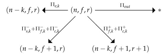
Figure 2.
The possible transitions when the retry limit is not reached.
- With probability , the process transits to the absorbing state .
- With probability , the slot is empty and k other STAs run out of energy. Thus, the process transits to .
- With probability , the slot is successful, the chosen STA does not try to transmit, and other STAs run out of energy; the process transits to .
- With probability , the slot is unsuccessful, the chosen STA does not try to transmit, and k other STAs run out of energy. The process transits to .
- With probability , the slot is collision, the chosen STA does not try to transmit, and k other STAs run out of energy. The process transits to .
- With probability , the chosen STA tries to transmit a frame, the slot is unsuccessful, and k other STAs run out of energy. The process transits to .
- With probability , the slot is collision, the chosen STA tries to transmit a frame, and k other STAs run out of energy. The process transits to .
If the STA’s retry counter r reaches RL, then the process transitions corresponding to the cases when the chosen STA tries to transmit, but the slot is unsuccessful (with probability ) or collision (with probability ) also leads to the absorbing state , as shown in Figure 3.
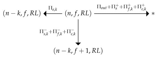
Figure 3.
The possible transitions when the retry limit is reached.
We need some auxiliary values to present the transition probabilities.
4.2.1. The Probability of Chosen STA Transmitting a Frame
We need to find the probability of the chosen STA to transmit a frame, provided that the slot number equals t, and the STA has made r transmission attempts. Let us define the following probabilities:
- is the probability of the considered process not to transit to the absorbing state and the chosen STA making r transmission attempts by the moment t.
- is the probability of the considered process by the moment t not to transit to the absorbing state, the chosen STA making r transmission attempts and an event occurring:
- –
- means that the STA makes a transmission attempt.
- –
- C means that the STA makes a transmission attempt that leads to collision.
- –
- S means that the STA makes a transmission attempt that does not lead to collision.
It is obvious that .
By definition, we have:
The numerator can be written as follows:
The first three equalities are obvious. The last one corresponds to transmission retries. After a collision or a frame being damaged by the noise, the STA chooses one of virtual slots, each with probability . The probability of transmission being disrupted by the noise equals . Then, the probability of collision or of the frame being damaged by noise equals .
Let us find . Note that the retry-counter equals r at the beginning of slot t if and only if it has turned r in one of the previous slots, and, since that moment, the chosen STA has not tried to transmit. In this case:
For an infinite number of STAs, the transmission probability equals the probability of collision: . Let us define values and , in which and turn when the number of STAs is infinite. These values are determined by the following formulae:
Instead of , we use its approximation , corresponding to the case, when the transmission probability equals the collision probability. In [27], it is shown that the error induced by such approximation is negligibly small even for STAs and decreases with the growth of N.
4.2.2. The Probability of Other STA Transmitting a Frame
Let us randomly choose an STA from those other STAs that are still alive by the slot t. Let us find the probability of this STA making a transmission attempt in instant t with given and . By definition
where is the probability of the considered process to be found in state at the moment t, and is the probability of considered process to be found in state at the moment t and the randomly chosen STA making a transmission attempt.
By the law of total probability,
It is obvious that the probability of an STA transmitting in slot t depends only on the slot number and on the number of its transmission attempts, i.e., . Let us replace with its approximate value and introduce a value
which approximates and coincides with it in case of the infinite number of STAs. The limits of summation over are explained by the fact that the number of retries does not exceed the number of non-empty slots and does not exceed the retry limit.
4.2.3. Additional Values
Let us introduce some more auxiliary values that determine the transmission probabilities in the state :
- is the probability of k other STAs transmitting in slot t,
- is the probability of none of the STAs transmitting in slot t,
- is the probability of only the chosen STA transmitting in slot t,
- is the probability of one other STA transmitting in slot t,
- is the probability of the chosen STA and at least one other STA transmitting in slot t,
- is the probability of the chosen STA not transmitting in slot t, but at least two other STAs transmitting in this slot.
These values by definition equal zero when . Let us express these values in terms of and :
For the purpose of brevity, we hereinafter omit the argument for probabilities of transmission and transition .
4.2.4. The Probability of the Process to Transit to the Absorbing State
We assume that the STA spends energy units in an empty slot, energy units in a successful slot if it does not transmit and energy units if it transmits, energy units in an unsuccessful or collision slot if it does not transmit and energy units if it transmits. The energy consumption values are calculated as follows:
where V is the voltage and , , are the current values, consumed by the STA while listening to the channel, receiving and transmitting, respectively.
The way the probability of transition to the absorbing state is calculated depends on the current state:
- If the STA cannot transmit the frame by the end of the RAW, i.e., , the process transits to the absorbing state, i.e., .
- Otherwise, two situations are possible:
- –
- if , the process transits to the absorbing state if the frame transmission is successful, or if the chosen STA runs out of energy:
- –
- if , the process transits to the absorbing state on any transmission attempt, or if the chosen STA runs out of energy:
Note that all other transitions take place only if .
4.2.5. The Probability of the Slot Being Empty
To find we take into account that none of the STAs access the channel and k other STAs run out of energy:
4.2.6. The Probability of the Slot Being Successful and the Chosen STA Not Trying to Transmit
After a successful transmission, the transmitting STA turns of, therefore more STAs, must run out of energy to make a total of k STAs that turn off by the end of the slot:
4.2.7. The Probability of the Slot Being Unsuccessful and the Chosen STA Not Trying to Transmit
If the transmitting STA has enough energy to transmit in the following slot, k STAs must run out of energy. Otherwise, only STAs must run out of energy:
4.2.8. The Probability of the Slot Being Collision and the Chosen STA Not Trying to Transmit
In the given formula, we sum over the number of STAs i that participate in the collision. For each i, we go over the number of STAs j that participate in the collision and run out of energy. If j STAs participating in the collision run out of energy, then STAs not participating in the collision must run out of energy too, i.e.,
4.2.9. The Probability of the Chosen STA Trying to Transmit and the Slot Being Unsuccessful
This event takes place when the chosen STA alone gains access to the channel, its transmission is disrupted by the noise, and it has already made transmission attempts. In addition, k other STAs have to run out of energy. The probability of this event equals:
4.2.10. The Probability of the Chosen STA Trying to Transmit and the Slot Being Collision
This transition takes place if . As in the case when the chosen STA does not transmit, we sum over the number i of STAs, taking part in the collision. The difference is that the lower limit of i is 1:
4.3. The Probability of the Chosen STA Transmitting Its Frame Successfully
The considered process in initially in state , where N is the initial number of STAs:
The possible transitions from state are shown in Figure 2 and Figure 3. Let us know the distribution for the moment t. Then, we can use the transition probabilities to calculate the distribution for the next time moment.
The probability of the chosen STA transmitting its frame successfully during the RAW is calculated as:
It is sufficient to sum over those t, for which because . Thus, to find , we consider the evolution of the transmission process starting with its initial state at time , and iteratively calculate the probability of the process to reach its possible states at time t until either the real time exceeds , or the total probability of the process to reach an absorbing state becomes close to 1. The calculations can be hastened by omitting the states with low (in comparison with the required accuracy) probability. We further use in Equation (2) to obtain the probability of successful transmission by the chosen STA in the RAW slot and further to find the optimal number of groups.
5. Numerical Results
In this section, we present and analyze the numerical results obtained using the designed models. In Section 5.1, we consider a single RAW slot and examine the dependence of the probability of successful transmission on different parameters, such as the average STA energy, probability of transmission being disrupted by noise, and the number of STAs. In Section 5.2, we consider the Periodic RAW and show the dependency of the amount of allocated channel resource on the number of groups.
5.1. RAW Slot
We assume that the STAs operate in a 2 MHz channel and use the most reliable modulation coding scheme (MCS0). The STAs transmit 100-byte data frames. Table 2 lists the experiment parameters. Specifically, the values of channel access parameters are given in the IEEE 802.11ah [10] amendment. Voltage V and the values of current , , , consumed by the STA while listening to the channel, receiving, and transmitting, respectively, are given in the IEEE simulation scenario recommendations [52].
Table 2.
Experiment parameters.
Figure 4 shows the dependency of the probability of successful frame transmission during the RAW slot on the RAW slot duration for various values of . The shown dependencies are monotonic, and the probability of success asymptotically approaches some value. This value is less than one because the STA’s energy is limited. In addition, this value decreases with an increase of N and p and with a decrease of . This result is expected because the greater initial number of STAs yields the greater probability of their frames to enter a collision, and retries, caused by the collisions or noise, result in higher energy consumption. As a result, the STA can deplete its energy before successful transmission.
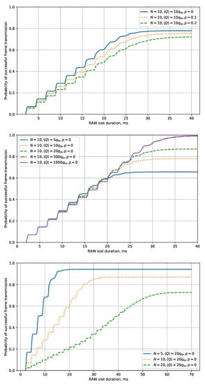
Figure 4.
The dependency of the probability of successful frame transmission on the RAW slot duration for various p, , and N.
Before the probability becomes constant, it grows “step-by-step” with the increase of the RAW slot duration. Such behavior is directly related to the fact that, with the increase of the RAW slot duration, the number of frames that can be transmitted within the RAW slot increases in a step-type manner. The width of a “step” is determined by the non-empty slot duration of and approximately equals . The height of a “step” is determined by the number of STAs N and the initial contention window . To find it, let us consider the beginning of the RAW slot and assume that all the STAs have sufficient energy to make the first transmission attempt. The first step of the plot corresponds to a situation when the chosen STA makes a successful first transmission attempt, and other STAs do not transmit their frames before the chosen STA. For slot number k, the probability of such an event equals
where the first multiplier is the probability of the chosen STA selecting the considered slot for transmission, and the expression in brackets is the probability that the other STAs select slots after the considered one. Summing over all k possible for the first transmission attempt, we obtain the step height:
The steps become more and more smooth with the increase of the RAW slot duration.
Let us find the minimal , which yields the required probability of successful transmission. This value may not exist if the average STA’s energy is too low, or there are too many STAs, or the noise level is too high. For example, in case , , , the probability of successful transmission of 0.9 cannot be achieved with any duration of RAW slot. However, with and , the required probability is reached with ms. Such a result shows the importance of the developed model: the models known from the literature, e.g., [27,49], do not consider the STA energy and would provide results similar to the results with a high . Thus, unlike the models known from the literature, the developed model shows us that, in some cases, we cannot achieve high probabilities of successful data transmission by increasing the RAW slot duration.
At the same time, the developed model gives us possible solutions for the considered case. The first one, if the considered devices gain energy from a renewable source (e.g., from a solar battery), is to delay the beginning of the RAW slot to let the STAs accumulate more energy, thus increasing . Another solution is to divide the STAs into two groups and thus to decrease the parameter N from 10 to 5. In such a case, the required probability of successful transmission becomes achievable with ms.
The grouping approach might be more efficient because the growth of the probability of successful transmission is not directly proportional to the number of STAs (see Figure 4).
5.2. Periodic RAW
Let us now investigate the case with periodic RAW. As a performance indicator of the network, we consider the cycle duration, which is the total duration of RAW slots (the numerator of the fraction in Equation (4)) within a single RAW period. The numerical results obtained for battery-powered energy harvesting STAs and are shown in Figure 5. We consider the values close to 100% within a small interval starting with 95%. The dependency of the cycle duration on the number of groups is non-monotonic, with extremum points corresponding to such numbers of groups by which the number of STAs is divisible. As one can see, a minimum minimorum exists that depends on the required probability of successful transmission .
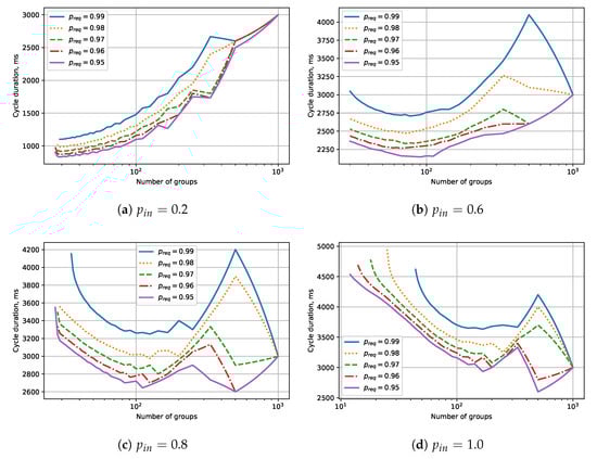
Figure 5.
The dependency of the cycle duration on the number of groups for different data generation probability .
The curves corresponding to different values converge when the number of groups equals the number of STAs. In this extreme case, every STA obtains a RAW slot, the length of which includes the time needed by the STA to count down its backoff and to transmit the frame. This length is the same for the considered values, and therefore the cycle durations are the same.
The important point is that small numbers of groups (and big numbers of STAs in a group) make the desired probability of success unachievable for any value of because STAs deplete their energy. Another point worth mentioning is that the cycle duration significantly depends on . Even though the considered values are close to 100%, even a 1% difference can bring a significant difference in the cycle duration. Specifically, with the increase of , it can suddenly change from increasing to decreasing dependency. This peculiarity is caused by the “step-by-step” dependency of the probability of successful transmission on the RAW duration.
To explain this fact, let us consider a case with and (see Figure 5d). If we divide STAs into 1000 groups, each group will contain exactly 1 STA. The duration of the RAW that each group obtains in the general case is determined by , but, for 1 STA, it equals for all considered values (see Figure 6). If we divide STAs into 500 groups, each group will contain exactly 2 STAs. In this case, the duration of the RAW slot varies significantly for different values. For , minimal RAW slot duration equals ms, so if we exchange two 1-STA groups for one 2-STA group, we win ms. However, for , minimal RAW slot duration equals ms, so, if we exchange two 1-STA groups for one 2-STA group, we lose ms.
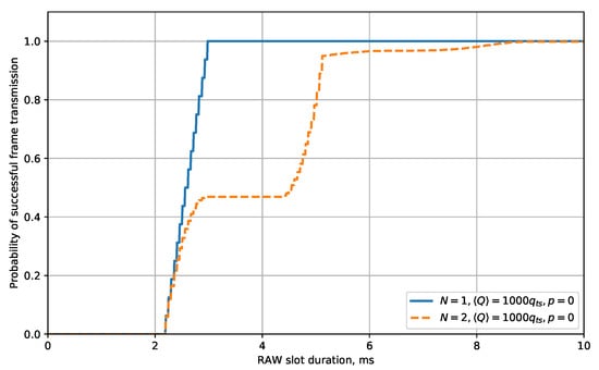
Figure 6.
The dependency of the probability of successful frame transmission on the RAW duration for small numbers of STAs.
6. Conclusions
Wi-Fi HaLow aims at extending the usage of Wi-Fi to the Internet of Things scenarios, which include gathering data from large numbers of autonomous energy-limited devices. An efficient tool that can help to reach this goal is the novel mechanism, introduced in the IEEE 802.11ah standard amendment: the Restricted Access Window (RAW). The Wi-Fi Access Point can use RAW to divide the connected STAs into groups and assign them a series of time intervals—RAW slots—during which only the STAs from a given group can transmit their data, thus decreasing the contention for channel access.
In the paper, we have studied an extreme scenario in which the STAs are energy-harvesting sensors that harvest energy with time and consume it during the data transmission, and it is possible that during the process of channel access and data transmission, the devices run out of energy. For such a scenario, we have developed an analytical model of data transmission that can be used to find the probability of successful data transmission by an STA as a function of the number of STAs, average STA energy, RAW slot duration, and the probability of a transmission to be damaged by random noise. Such a model can be used to determine the minimal RAW duration that, for a given number of STAs, can guarantee the given probability of data delivery. Unlike the existing models that do not take into account the energy consumption of devices, the developed model shows that, in some cases, the required probability of data delivery cannot be achieved by increasing the RAW slot duration. We have used this model to solve the STA grouping problem: how to divide the STAs into groups in such a way that all the STAs can transmit their data with required probability, and the portion of consumed channel resources is minimal. While solving the STA grouping problem, we have obtained and explained some paradoxical results, e.g., increasing the number of groups and correspondingly decreasing the number of STAs per group does not necessarily provide lower channel resource consumption. At the same time, the model can be used to find the optimal number of groups and the corresponding duration of RAW slots for each group which can decrease the cycle duration by almost 50% in comparison with the usage of a single group for all devices or with the usage of a group for each device.
Let us summarize the contributions of the paper:
- We have developed a model of data transmission in the RAW slot when STAs transmit single packets, the STAs have limited amounts of energy, and their transmissions can be disrupted by random noise. The model allows us to calculate the probability that the data are delivered with a given RAW configuration.
- We have shown that it is important to consider the amount of STAs’ energy in order to properly configure the RAW parameters, while the usage of models that do not consider the STA energy consumption may violate the requirements on the reliability of communications.
- We have shown how to use the developed model to optimize the RAW slot duration in order to provide the required probability of data delivery and to minimize the amount of consumed channel resources.
- We have shown that the channel resource consumption can change drastically depending on the reliability requirements: changing the required probability by 1% can increase the consumption by almost 100%, so the RAW parameters optimization shall take into account the requirements of particular applications.
As a direction of future work, we consider the modeling of data transmission for more complex models of traffic and energy harvesting. We also plan to consider the usage of RAW in heterogeneous networks.
Author Contributions
Conceptualization, E.K. and A.L.; Formal analysis, D.B. and E.K.; Investigation, E.K., A.L. and J.F.; Methodology, D.B. and E.K.; Software, D.B. and J.F.; Validation, D.B. and A.L.; Writing—original draft, D.B.; Writing—review and editing, E.K., A.L. and J.F. All authors read and agreed to the published version of the manuscript.
Funding
The research has been supported by the Russian Foundation for Basic Research (Grant No. 18-37-20077 mol-a-ved) and by the Flemish FWO SBO S004017N IDEAL-IoT (Intelligent DEnse and Long range IoT networks) project.
Conflicts of Interest
The authors declare no conflict of interest. The funders had no role in the design of the study; in the collection, analyses, or interpretation of data; in the writing of the manuscript, or in the decision to publish the results.
Abbreviations
The following abbreviations are used in this manuscript:
| ACK | Acknowledgement Frame |
| AIFS | Arbitration Inter-Frame Space |
| AP | Access Point |
| CSMA/CA | Carrier Sense Multiple Access with Collision Avoidance |
| EDCA | Enhanced Distributed Channel Access |
| IoT | Internet of Things |
| RAW | Restricted Access Window |
| SIFS | Short Inter-Frame Space |
| STA | Station |
References
- Atzori, L.; Iera, A.; Morabito, G. The Internet of Things: A Survey. Comput. Netw. 2010, 54, 2787–2805. [Google Scholar] [CrossRef]
- Cisco Internet of Things (IoT). Available online: http://www.cisco.com/web/solutions/trends/iot/overview.html (accessed on 20 April 2020).
- Prasad, R.V.; Devasenapathy, S.; Rao, V.S.; Vazifehdan, J. Reincarnation in the Ambiance: Devices and Networks with Energy Harvesting. IEEE Commun. Surv. Tutor. 2013, 16, 195–213. [Google Scholar] [CrossRef]
- Kosunalp, S. MAC Protocols for Energy Harvesting Wireless Sensor Networks: Survey. ETRI J. 2015, 37, 804–812. [Google Scholar] [CrossRef]
- Delgado, C.; Sanz, J.M.; Famaey, J. On the Feasibility of Battery-Less LoRaWAN Communications using Energy Harvesting. In Proceedings of the 2019 IEEE Global Communications Conference (GLOBECOM), Waikoloa, HI, USA, 9–13 December 2019; pp. 1–6. [Google Scholar]
- Orfei, F.; Mezzetti, C.B.; Cottone, F. Vibrations Powered LoRa Sensor: An Electromechanical Energy Harvester Working on a Real Bridge. In Proceedings of the 2016 IEEE SENSORS, Orlando, FL, USA, 30 October–3 November 2016; pp. 1–3. [Google Scholar]
- Loubet, G.; Takacs, A.; Gardner, E.; De Luca, A.; Udrea, F.; Dragomirescu, D. LoRaWAN Battery-Free Wireless Sensors Network Designed for Structural Health Monitoring in the Construction Domain. Sensors 2019, 19, 1510. [Google Scholar] [CrossRef] [PubMed]
- Fraternali, F.; Balaji, B.; Agarwal, Y.; Benini, L.; Gupta, R. Pible: Battery-Free Mote for Perpetual Indoor BLE Applications. In Proceedings of the 5th Conference on Systems for Built Environments, Shenzhen, China, 7–8 November 2018; pp. 168–171. [Google Scholar]
- Dekimpe, R.; Xu, P.; Schramme, M.; Gérard, P.; Flandre, D.; Bol, D. A Battery-Less BLE Smart Sensor for Room Occupancy Tracking Supplied by 2.45-GHz Wireless Power Transfer. Integration 2019, 67, 8–18. [Google Scholar] [CrossRef]
- IEEE. IEEE P802.11ahTM Standard for Information Technology—Telecommunications and Information Exchange between Systems Local and Metropolitan Area Networks—Specific Requirements—Part 11: Wireless LAN Medium Access Control (MAC) and Physical Layer (PHY) Specifications—Amendment 2: Sub 1 GHz License Exempt Operation; IEEE: Piscataway, NJ, USA, 2017. [Google Scholar]
- Khorov, E.; Lyakhov, A.; Krotov, A.; Guschin, A. A Survey on IEEE 802.11ah: An Enabling Networking Technology for Smart Cities. Comput. Commun. 2015, 58, 53–69. [Google Scholar] [CrossRef]
- Hester, J.; Sorber, J. The Future of Sensing is Batteryless, Intermittent, and Awesome. In Proceedings of the 15th ACM Conference on Embedded Network Sensor Systems, Delft, The Netherlands, 5–8 November 2017; pp. 1–6. [Google Scholar]
- Shirvanimoghaddam, M.; Shirvanimoghaddam, K.; Abolhasani, M.M.; Farhangi, M.; Barsari, V.Z.; Liu, H.; Dohler, M.; Naebe, M. Towards a Green and Self-Powered Internet of Things using Piezoelectric Energy Harvesting. IEEE Access 2019, 7, 94533–94556. [Google Scholar] [CrossRef]
- Ye, W.; Heidemann, J.; Estrin, D. An Energy-Efficient MAC Protocol for Wireless Sensor Networks. In Proceedings of the INFOCOM 2002, Twenty-First Annual Joint Conference of the IEEE Computer and Communications Societies, New York, NY, USA, 23–27 June 2002; Volume 3, pp. 1567–1576. [Google Scholar]
- Lee, K.; Lee, J.; Yi, Y.; Rhee, I.; Chong, S. Mobile Data Offloading: How Much can WiFi Deliver? IEEE/ACM Trans. Networking 2010, 21, 536–550. [Google Scholar] [CrossRef]
- Tian, L.; Khorov, E.; Latré, S.; Famaey, J. Real-Time Station Grouping under Dynamic Traffic for IEEE 802.11ah. Sensors 2017, 17, 1559. [Google Scholar] [CrossRef]
- Šljivo, A.; Kerkhove, D.; Tian, L.; Famaey, J.; Munteanu, A.; Moerman, I.; Hoebeke, J.; De Poorter, E. Performance Evaluation of IEEE 802.11ah Networks with High-Throughput Bidirectional Traffic. Sensors 2018, 18, 325. [Google Scholar] [CrossRef]
- Raeesi, O.; Pirskanen, J.; Hazmi, A.; Levanen, T.; Valkama, M. Performance Evaluation of IEEE 802.11ah and its Restricted Access Window Mechanism. In Proceedings of the 2014 IEEE international conference on communications workshops (ICC), Sydney, Australia, 10–14 June 2014; pp. 460–466. [Google Scholar]
- Hazmi, A.; Badihi, B.; Larmo, A.; Torsner, J.; Valkama, M.; Qutab-ud-din, M. Performance Analysis of IoT-Enabling IEEE 802.11ah Technology and its RAW Mechanism with non-Cross Slot Boundary Holding Schemes. In Proceedings of the 2015 IEEE 16th International Symposium on a World of Wireless, Mobile and Multimedia Networks (WoWMoM), Boston, MA, USA, 14–17 June 2015; pp. 1–6. [Google Scholar]
- Nawaz, N.; Hafeez, M.; Zaidi, S.A.R.; McLernon, D.C.; Ghogho, M. Throughput Enhancement of Restricted Access Window for Uniform Grouping Scheme in IEEE 802.11ah. In Proceedings of the 2017 IEEE International Conference on Communications (ICC), Paris, France, 21–25 May 2017; pp. 1–7. [Google Scholar]
- Madueño, G.C.; Stefanović, Č.; Popovski, P. Reliable and Efficient Access for Alarm-Initiated and Regular M2M Traffic in IEEE 802.11ah Systems. IEEE Internet Things J. 2015, 3, 673–682. [Google Scholar] [CrossRef]
- Wang, Y.; Chai, K.K.; Chen, Y.; Schormans, J.; Loo, J. Energy-Aware Restricted Access Window Control with Retransmission Scheme for IEEE 802.11ah (Wi-Fi HaLow) Based Networks. In Proceedings of the 2017 13th Annual Conference on Wireless On-demand Network Systems and Services (WONS), Jackson, WY, USA, 21–24 February 2017; pp. 69–76. [Google Scholar]
- Bel, A.; Adame, T.; Bellalta, B. An Energy Consumption Model for IEEE 802.11ah WLANs. Ad Hoc Netw. 2018, 72, 14–26. [Google Scholar] [CrossRef]
- Ali, M.Z.; Mišić, J.; Mišić, V.B. Efficiency of Restricted Access Window Scheme of IEEE 802.11ah under non-Ideal Channel Condition. In Proceedings of the 2018 IEEE International Conference on Internet of Things (iThings) and IEEE Green Computing and Communications (GreenCom) and IEEE Cyber, Physical and Social Computing (CPSCom) and IEEE Smart Data (SmartData), Halifax, NS, Canada, 30 July–3 August 2018; pp. 251–256. [Google Scholar]
- Ali, M.Z.; Mišić, J.; Mišić, V.B. Performance Evaluation of Heterogeneous IoT Nodes with Differentiated QoS in IEEE 802.11ah RAW Mechanism. IEEE Trans. Veh. Technol. 2019, 68, 3905–3918. [Google Scholar] [CrossRef]
- Kai, C.; Zhang, J.; Zhang, X.; Huang, W. Energy-Efficient Sensor Grouping for IEEE 802.11ah Networks with Max-Min Fairness Guarantees. IEEE Access 2019, 7, 102284–102294. [Google Scholar] [CrossRef]
- Khorov, E.; Krotov, A.; Lyakhov, A. Modelling Machine Type Communication in IEEE 802.11ah. In Proceedings of the IEEE International Conference on Communications (ICC), London, UK, 8–12 June 2015. [Google Scholar]
- Khorov, E.; Krotov, A.; Lyakhov, A.; Yusupov, R.; Condoluci, M.; Dohler, M.; Akyildiz, I. Enabling the Internet of Things with Wi-Fi Halow—Performance Evaluation of the Restricted Access Window. IEEE Access 2019, 7, 127402–127415. [Google Scholar] [CrossRef]
- Khorov, E.; Lyakhov, A.; Yusupov, R. Two-Slot Based Model of the IEEE 802.11ah Restricted Access Window with Enabled Transmissions Crossing Slot Boundaries. In Proceedings of the 2018 IEEE 19th International Symposium on “A World of Wireless, Mobile and Multimedia Networks” (WoWMoM), Chania, Greece, 12–15 June 2018; pp. 1–9. [Google Scholar]
- Bhandari, S.; Sharma, S.K.; Wang, X. Device Grouping for Fast and Efficient Channel Access in IEEE 802.11ah Based IoT Networks. In Proceedings of the 2018 IEEE International Conference on Communications Workshops (ICC Workshops), Kansas City, MO, USA, 20–24 May 2018; pp. 1–6. [Google Scholar]
- Akan, O.B.; Cetinkaya, O.; Koca, C.; Ozger, M. Internet of Hybrid Energy Harvesting Things. IEEE Internet Things J. 2017, 5, 736–746. [Google Scholar] [CrossRef]
- Eu, Z.A.; Tan, H.P.; Seah, W.K. Design and Performance Analysis of MAC Schemes for Wireless Sensor Networks Powered by Ambient Energy Harvesting. Ad Hoc Netw. 2011, 9, 300–323. [Google Scholar] [CrossRef]
- Lee, P.; Eu, Z.A.; Han, M.; Tan, H.P. Empirical Modeling of a Solar-Powered Energy Harvesting Wireless Sensor Node for Time-Slotted Operation. In Proceedings of the 2011 IEEE wireless communications and networking conference, Cancun, Mexico, 28–31 March 2011; pp. 179–184. [Google Scholar]
- Liu, W.; Zhou, X.; Durrani, S.; Mehrpouyan, H.; Blostein, S.D. Energy Harvesting Wireless Sensor Networks: Delay Analysis Considering Energy Costs of Sensing and Transmission. IEEE Trans. Wirel. Commun. 2016, 15, 4635–4650. [Google Scholar] [CrossRef]
- Mahdavi-Doost, H.; Yates, R.D. Energy Harvesting Receivers: Finite Battery Capacity. In Proceedings of the 2013 IEEE International Symposium on Information Theory, Istanbul, Turkey, 7–12 July 2013; pp. 1799–1803. [Google Scholar]
- Ventura, J.; Chowdhury, K. Markov Modeling of Energy Harvesting Body Sensor Networks. In Proceedings of the 2011 IEEE 22nd International Symposium on Personal, Indoor and Mobile Radio Communications, Toronto, ON, Canada, 11–14 September 2011; pp. 2168–2172. [Google Scholar]
- Gelenbe, E. A Sensor Node with Energy Harvesting. ACM SIGMETRICS Perform. Eval. Rev. 2014, 42, 37–39. [Google Scholar] [CrossRef]
- Gelenbe, E.; Ceran, E.T. Energy Packet Networks with Energy Harvesting. IEEE Access 2016, 4, 1321–1331. [Google Scholar] [CrossRef]
- Abdelrahman, O.H.; Gelenbe, E. A Diffusion Model for Energy Harvesting Sensor Nodes. In Proceedings of the 2016 IEEE 24th International Symposium on Modeling, Analysis and Simulation of Computer and Telecommunication Systems (MASCOTS), London, UK, 19–21 September 2016; pp. 154–158. [Google Scholar]
- Yang, Z.; Xu, W.; Pan, Y.; Pan, C.; Chen, M. Energy Efficient Resource Allocation in Machine-to-Machine Communications with Multiple Access and Energy Harvesting for IoT. IEEE Internet Things J. 2017, 5, 229–245. [Google Scholar] [CrossRef]
- Yang, Z.; Xu, W.; Pan, Y.; Pan, C.; Chen, M. Optimal Fairness-Aware Time and Power Allocation in Wireless Powered Communication Networks. IEEE Trans. Commun. 2018, 66, 3122–3135. [Google Scholar] [CrossRef]
- Haridas, A.; Rao, V.S.; Prasad, R.; Sarkar, C. Opportunities and Challenges in Using Energy-Harvesting for NB-IoT. ACM SIGBED Rev. 2018, 15, 7–13. [Google Scholar] [CrossRef]
- Bouguera, T.; Diouris, J.F.; Chaillout, J.J.; Jaouadi, R.; Andrieux, G. Energy Consumption Model for Sensor Nodes Based on LoRa and LoRaWAN. Sensors 2018, 18, 2104. [Google Scholar] [CrossRef] [PubMed]
- Sherazi, H.H.R.; Imran, M.A.; Boggia, G.; Grieco, L.A. Energy Harvesting in LoRaWAN: A Cost Analysis for the Industry 4.0. IEEE Commun. Lett. 2018, 22, 2358–2361. [Google Scholar] [CrossRef]
- Amaro, J.P.; Ferreira, F.J.; Cortesão, R.; Landeck, J. Energy Harvesting for ZigBee Compliant Wireless Sensor Network Nodes. In Proceedings of the IECON 2012-38th Annual Conference on IEEE Industrial Electronics Society, Montreal, QC, Canada, 25–28 October 2012; pp. 2583–2588. [Google Scholar]
- Bankov, D.; Khorov, E.; Lyakhov, A.; Stepanova, E. IEEE 802.11ba—Extremely Low Power Wi-Fi for Massive Internet of Things—Challenges, Open Issues, Performance Evaluation. In Proceedings of the 2019 IEEE International Black Sea Conference on Communications and Networking (BlackSeaCom), Sochi, Russia, 3–6 June 2019; pp. 1–5. [Google Scholar]
- Froytlog, A.; Foss, T.; Bakker, O.; Jevne, G.; Haglund, M.A.; Li, F.Y.; Oller, J.; Li, G.Y. Ultra-Low Power Wake-up Radio for 5G IoT. IEEE Commun. Mag. 2019, 57, 111–117. [Google Scholar] [CrossRef]
- Bianchi, G. Performance Analysis of the IEEE 802.11 Distributed Coordination Function. Sel. Areas Commun. IEEE J. 2000, 18, 535–547. [Google Scholar] [CrossRef]
- Khorov, E.; Lyakhov, A.; Nasedkin, I.; Yusupov, R.; Famaey, J.; Akyildiz, I. Fast and Reliable Alert Delivery in Mission-Critical Wi-Fi HaLow Sensor Networks. IEEE Access 2020, 8, 14302–14313. [Google Scholar] [CrossRef]
- Vishnevsky, V.; Lyakhov, A. 802.11 LANs: Saturation Throughput in the Presence of Noise. In Networking 2002: Networking Technologies, Services, and Protocols; Performance of Computer and Communication Networks; Mobile and Wireless Communications; Springer: Berlin/Heidelberg, Germany, 2002; pp. 1008–1019. [Google Scholar]
- Nasir, A.A.; Zhou, X.; Durrani, S.; Kennedy, R.A. Wireless-Powered Relays in Cooperative Communications: Time-Switching Relaying Protocols and Throughput Analysis. IEEE Trans. Commun. 2015, 63, 1607–1622. [Google Scholar] [CrossRef]
- TGax Simulation Scenarios. Available online: https://mentor.ieee.org/802.11/dcn/14/11-14-0980-10-00ax-simulation-scenarios.docx (accessed on 20 April 2020).


© 2020 by the authors. Licensee MDPI, Basel, Switzerland. This article is an open access article distributed under the terms and conditions of the Creative Commons Attribution (CC BY) license (http://creativecommons.org/licenses/by/4.0/).