1. Introduction
Coastal wetlands, which play a significant role in protecting biodiversity, controlling runoff and regulating climate [
1,
2], are some of the most heavily used and threatened natural systems. Due to the complex ecological conditions of wetlands and the spatial and temporal limitations of field investigations, remote sensing technology has become an important means of wetland mapping and monitoring. Despite the success of optical satellite data in applications such as wetland detection and water level monitoring [
3,
4,
5], optical images are less useful in coastal areas due to cloud cover [
6]. Synthetic Aperture Radar (SAR), which provides valuable geophysical parameters over intertidal zones in all-weather and daylight-independent conditions [
7,
8,
9], has emerged as a promising tool for wetland monitoring. In particular, quad-polarized data can provide more details to meet the requirements for wetland classification, and various polarization decomposition methods have been demonstrated to provide abundant polarization features, which improve the classification precision [
10,
11,
12].
Gaofen-3 (GF-3), launched on 10 August 2016, is the first Chinese civilian satellite to be equipped with multi-polarized C-band SAR at the meter-level resolution [
13]. The SAR payload can support observations in single-, dual- and quad-polarization modes, and its products can be used in marine environmental monitoring, resource surveys and disaster prevention [
14]. In recent years, the advantages of SAR data with high spatial resolution from a variety of satellites, such as RADARSAT-2 [
15,
16], Sentinel-1 [
17] and ALOS-2 [
18], have been demonstrated in different applications. However, the usage of GF-3 data is very low, which is likely related to its recent launch date [
19]. Coastal wetland classification with GF-3 polarimetric SAR imagery remains a challenge. Currently, only Yellow River Delta has the application with GF-3 data [
20], while the Yancheng coastal wetlands have not been discussed. The selection of an appropriate SAR wavelength is one of the vital influential factors for land cover classification [
21]. In general, the use of X- and C-bands is preferred for herbaceous wetlands and less dense canopies, while L-band is preferred for woody wetlands, such as swamps and other wetland classes with high biomass [
22]. Magaly et al. [
23] evaluated the contributions of Radarsat-2 (C-band) and ALOS\PALSAR (L-band) full polarimetric data in characterizing and mapping wetland conditions, and found that the variations in canopy structures were better discriminated with C-band than L-band data, while L-band data was useful in determining the wetness conditions of the ground surface. Other studies have demonstrated that shorter wavelengths, such as C-band and X-band, are better suited for non-forested wetlands vegetation patterns, such as bogs, fens and marshes [
24,
25]. The Yancheng coastal wetlands, which provide important ecosystem services to local communities, consist primarily of extensive intertidal mudflats, river channels, salt marshes, reed beds and marshy grasslands. Therefore, GF-3 equipped with C-band SAR probably has great potential for coastal wetland mapping in this region, and this article will explore the use of C-band fully polarimetric GF-3 image for wetland classification in the Yancheng coastal development zone of Jiangsu Province, China.
Some studies that used fully polarimetric SAR imagery have noted the influence of different polarimetric scattering features on wetland classification results [
26,
27]. For example, Millard et al. combined SAR and Lidar data to achieve higher accuracy [
28]. Chen et al. integrated 20 polarimetric decomposition algorithms and proposed a feature set optimization method to select the optimal polarimetric features for wetland classification [
29]. However, these studies only improved the feature optimization method from a statistical perspective and did not consider the applicability of the features to wetland identification. Other studies have evaluated the importance of different polarization decomposition models in wetland identification. For example, features from the Cloude–Pottier and Freeman–Durden methods were determined to be the best for discriminating land types in wetlands when using RADARSAT-2 data [
30,
31]. However, they just discussed the influence of features on the wetland classification result according to the overall classification accuracy, while ignoring the influence of features on the classification accuracy of typical wetland vegetation. Especially, Neumann decomposition has been proved useful in crop classification [
32], but whether it is suitable for wetland classification has not been discussed.
In this research, we aimed to apply GF-3 data to coastal wetland classification. For this purpose, the eastern coastal wetland of Jiangsu, China, was taken as the study area. The specific objectives of this research were (1) to test the validity of using GF-3 polarimetric SAR imagery to classify coastal wetlands with an object-oriented random forest algorithm; (2) to integrate three frequently used polarimetric decomposition algorithms to extract polarimetric scattering features and propose a feature set optimization method; and (3) to investigate the influence of polarization features on the discrimination of typical land cover types in wetlands, especially different wetland vegetation in coastal tidal flats.
The rest of this paper is structured as follows:
Section 2 introduces the study site, reference data and satellite imagery in this research.
Section 3 provides a description of the methodology.
Section 4 presents the experimental results and discussion. Finally, conclusions and perspectives for future work are outlined in
Section 5.
4. Results and Discussion
4.1. Importance of Polarization Features for Wetland Classification
Figure 4 shows the MDA of each feature after adding noise to it. The most discriminating features were SE, Y4_Vol, Span and Neu_tau, which had MDA values of 0.247, 0.213, 0.169 and 0.124. The least discriminating features were Neu_psi, Neu_mod and α, the MDA values of which were less than 0.05.
To explore the influence of each feature on classification, we also calculated MDA values for each feature in every category.
The statistical results for non-vegetation are shown in
Figure 5a–c. The results clearly show that SERD was the most important feature for the beach, with an MDA of 0.012, followed by SE and Neu_tau, which had little effect, with an MDA of less than 0.01. In the classification of water, Span, SE and Y4_Odd were the most important features, with an MDA of 0.0394, 0.0254 and 0.0247. In the classification of road, H and SE were the most important features; their MDA values were 0.0418 and 0.0416.
As shown in
Figure 5d,e, SE and Span were the most effective features for typical wetland vegetation. In the classification of
Suaeda salsa, the three most important features were Neu_tau, SE and Span; their MDA values were 0.0599, 0.0536 and 0.0462. In the classification of
Spartina alterniflora, the three most effective features were Span, SE and A, with MDA values of 0.0722, 0.0687 and 0.0677.
As shown in
Figure 5f,g, the classification of irrigable land and rice paddy was differently affected by the features. For irrigable land, Y4_Vol, Y4_Dbl and Neu_tau were the most discriminating features, and their MDA values were 0.0522, 0.0386 and 0.0356. For rice paddy, Neu_tau, Span and SE were the three most discriminating features, with an MDA of 0.0628, 0.0607 and 0.0543.
4.2. Discussion on Different Polarization Features in Typical Wetland Classes
The experimental results in
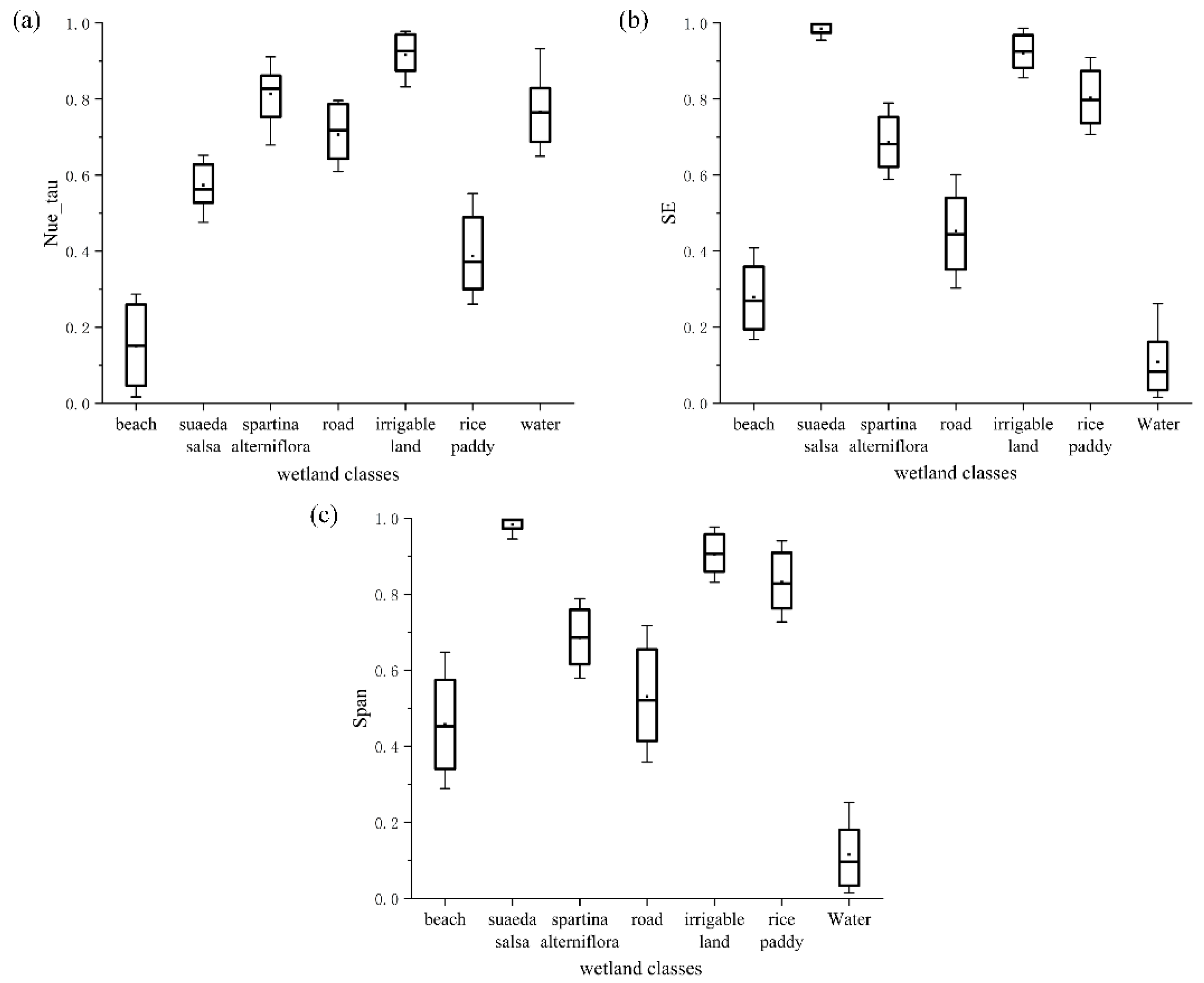
Section 4.1 demonstrate that SE, Neu_tau and Span are key features that affect wetland classification. Boxplots were used to analyze and understand the mechanism of each feature for each land cover.
As observed in
Figure 6a, the value of Neu_tau was lowest for the beach and highest for irrigable land, and the feature distribution intervals of Neu_tau for
Suaeda salsa and rice paddy differed from those of other classes. Therefore, Neu_tau can effectively distinguish between the above categories. As revealed in
Figure 6b, the value of SE was the lowest for water and the highest for
Suaeda salsa. Furthermore, the SE values were quite different between categories. Thus, SE is highly important in all categories. As shown in the boxplot, the value of Span for water was significantly lower than for the other categories, so Span is particularly important in water classification.
4.3. Classification Comparison
Different feature sets were constructed in order to compare their effects. The statistical accuracy was the highest when seven features were used. Therefore, seven features with the highest impact on the classification were selected to build the feature set (FS). Different feature sets were constructed to compare the results of different decomposition methods. Combining Span and features from Cloude–Pottier decomposition was always important in wetland classification [
11]. In these experiments, when Span was used with features from Cloude–Pottier decomposition, the feature set H/A/span was the best combination. Similarly, Neu_mod and Neu_pha from Neumann decomposition obtained the best classification accuracy when combined with span. Thus, the feature set Neu_mod/Nue_pha/span was used to evaluate the effectiveness of the Neumann decomposition in wetland classification. The features from Yamaguchi decomposition showed high importance, so a feature set named Y4 was constructed with these features. To evaluate the effect of feature optimization, the original feature set with all 16 features, designated ALL, was tested. To illustrate the effectiveness of the method, feature set ALL also be employed by SVM.
The results are shown in
Figure 7. As illustrated in
Figure 7b, the feature set H/A/span misclassified rice paddy as
Spartina alterniflora, and the extraction of
Suaeda salsa was incomplete. With the use of Neu_tua/Neu_pha/span in
Figure 7c, rice paddy and
Ssuaeda salsa were more complete, but the misclassification of rice paddy and
Spartina alterniflora was worse. The results for Y4 are shown in
Figure 7d, which shows that the misclassification of rice paddy and
Spartina alterniflora decreased, and the extraction of
Suaeda salsa and rice paddy was more complete. However, part of irrigable land was misclassified as
Suaeda salsa.
Figure 7e shows the result of using all the features for classification; the results improved, but the rice paddy was fragmentized.
Figure 7f shows the result of using all the features by SVM, the misclassification was more serious than
Figure 7e. As revealed in
Figure 7a, when three key features were added to Y4, the confusion between
Suaeda salsa and irrigable land decreased, and the rice paddy results improved. The boundaries between classes were clear, and the best effect on classification was obtained. In addition,
Figure 7 shows that the mapping result for the beach was unsatisfactory and fragmentized. The reason for this is that the data was captured at 3 a.m., which coincided with the ebb tide. The receding tide covered most of the beach.
In order to further evaluate each feature set, the overall accuracy and kappa coefficient of each result were calculated. The results are shown in
Table 3, and the confusion matrixes are shown in
Table 4,
Table 5,
Table 6,
Table 7,
Table 8 and
Table 9.
Table 3 shows that the overall accuracy and kappa coefficient were the lowest when using the feature set H/A /span, with values of 77.80% and 0.7319. When the feature set Neu_tua/Neu_pha/span was used for classification, the overall accuracy and kappa coefficient rose to 82.93% and 0.7962. When features from the Yamaguchi decomposition were used, the overall accuracy and kappa coefficient were improved to 87.94% and 0.859. To some extent, this suggests that Yamaguchi decomposition was more effective than Cloude–Pottier and Neumann decompositions in coastal wetland classification. When all the features were used in the classification, the overall accuracy and kappa coefficient were 89.24% and 0.87. When the feature set was reduced to FS, the overall accuracy and kappa coefficient were the highest (92.86% and 0.914). This illustrates the significance of feature optimization. When the feature set ALL was used in random forest and SVM, the accuracy dropped from 89.94% to 85.57%, and the Kappa coefficient dropped from 0.87 to 0.8269. This shows the superiority of random forest over SVM.
4.4. Discussion
With the algorithm constructed in this study, SE, Y4_Vol, Span, Neu_tau, Y4_Dbl, Y4_Odd and Y4_Hlx were found to be the most important parameters for wetland classification. The classification accuracy of this optimized feature set was 92.86%, which is higher than that of the original feature set, the accuracy of which was 89.24%. This suggests that feature redundancy occurs when too many features are included in the feature set. Moreover, features with a low classification ability may even cause noise and affect the result.
In general, SE, Y4_Vol, Span and Neu_tau had the most significant influence on wetland classification. Among these features, Neu_tau was highly effective in distinguishing vegetation, Span could markedly improve the mixture of beach and water, and SE could distinguish each class and improve the classification as a whole.
By adding white noise to each feature, MDA was calculated for every class, and the sequence of importance was obtained for each land cover type. Suaeda salsa and Spartina alterniflora are typical species of wetland vegetation at the study site. Neu_tau, SE and Span were the most important features for the classification of Suaeda salsa, and Span, SE and A were the most discriminating features for Spartina alterniflora.
In the three decomposition methods used in the study, the parameters obtained from the Yamaguchi decomposition were the most appropriate for wetland mapping. All of the parameters obtained from Yamaguchi decomposition were highly important for wetland classification. Yamaguchi decomposition was generally effective in classifying the wetland, and the accuracy was 87.94%. Although some parameters from the Neumann and Cloude–Pottier decompositions were correlative, the feature set from Neumann decomposition combined with Span had a higher accuracy than that from the Cloude–Pottier decomposition with Span. This indicates that some features from the Neumann decomposition are more appropriate for wetland mapping than those from the Cloude–Pottier decomposition.
Despite the significant importance of Neu_tau in coastal wetland classification, some features, such as Neu_mod and Neu_pis, were incapable of discriminating between categories. Therefore, feature screening is necessary when using multiple decomposition methods.
To illustrate the effectiveness of the method, the classification results of SVM and random forest are shown in
Figure 7, and the accuracy and Kappa coefficients are showed in
Table 3,
Table 4,
Table 5,
Table 6,
Table 7,
Table 8 and
Table 9. When the same feature sets were employed for the classification, the results of RF were superior to the result of SVM. To some extent, this demonstrated the effectiveness of the classifier in the method proposed in the paper. Comparing the results of the optimal feature set and the feature set without optimization, the result of FS was superior than ALL. This demonstrated the utility of the proposed feature set optimization method.
The method proposed in this paper is not only applicable to wetland classification, but also has universal applicability in other land cover classifications, such as for forests, urban areas, crops and so on. As is known to all, features are the basis of classification. The result of the selection of features will affect the result of the classification. This paper took wetlands as the study object, and better classification results were obtained from the classifier and feature selection. Therefore, it is reasonable to believe this method can be applied to other land cover classifications as well.
5. Conclusions
SAR image has become an important means of wetland research, but studies using GF-3 data for wetland classification are scarce. Furthermore, in feature set optimization, analyzing the influence of features on the basis of only the accuracy of wetland classification cannot meet the needs of this type of research. Therefore, in this research, fully polarimetric GF-3 data were used to study the classification of coastal wetlands, determine the influence of different polarization characteristics on wetland classification and identify typical features. The following conclusions can be drawn on the basis of experiments:
- (1)
GF-3 data provide rich and effective observation information, which can be used as a basis for wetland classification. The classification accuracy in this study reaches 92.86%.
- (2)
SE, Span, Y4_Vol and Neu_Tau play key roles in the classification of the wetland in this study. Among these features, SE improves the accuracy as a whole, and Neu_tau and Span are the most discriminating features for crops.
- (3)
For typical wetland vegetation, the most discriminative features are Neu_tau and SE for Suaeda salsa and Span and SE for Spartina alterniflora.
- (4)
Compared with the Cloude–Pottier and Neumann decompositions, Yamguchi decomposition is more effective in coastal wetland classification with GF-3 images.
Overall, the findings in this paper demonstrate that the presented feature set optimization method has significant advantages in coastal wetland classification when using fully polarimetric GF-3 data. However, there was some misclassification between rice paddy and Spartina alterniflora. Additionally, the feature set used in the study only included polarization features and not objected-oriented shape features, so it did not distinguish between the river and the fishpond. Future studies should employ other objected-oriented features or integrate optical and SAR data to distinguish between these two land cover types.


