
Dynamic Model of a Humanoid Exoskeleton of a Lower Limb with Hydraulic Actuators


Abstract
:1. Introduction
2. Materials and Methods
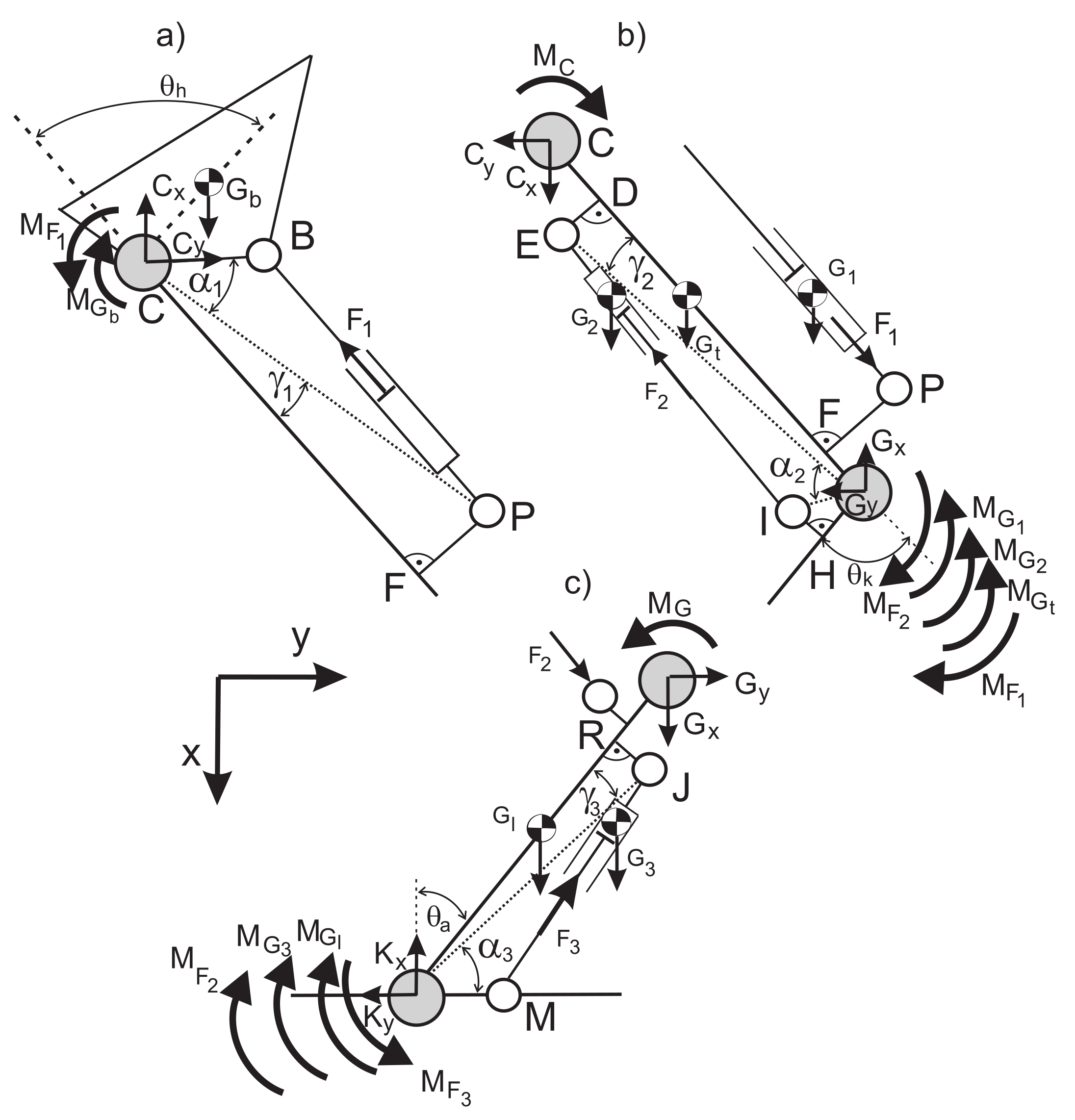
2.1. Exoskeleton Scheme
2.2. Coordinates
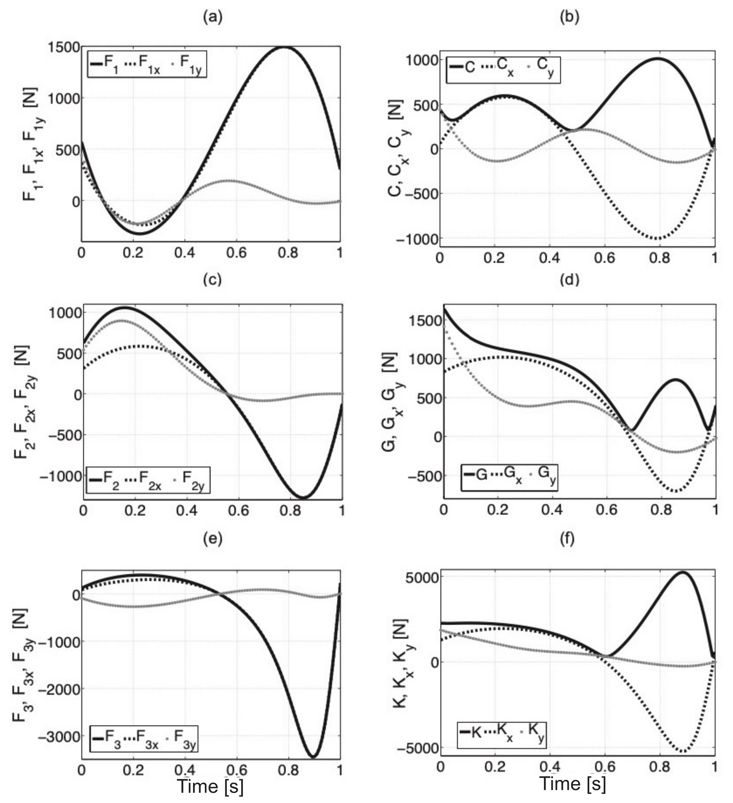
3. Results
4. Discussion
Author Contributions
Funding
Institutional Review Board Statement
Informed Consent Statement
Data Availability Statement
Acknowledgments
Conflicts of Interest
Abbreviations
| dimensions of the exoskeleton segments, | |
| dimensions of the exoskeleton segments, | |
| dimensions of the exoskeleton segments, | |
| foot length, | |
| shank length, | |
| thigh length, | |
| p | oil pressure, |
| W | user height, |
| actuator forces, | |
| , | components of hip forces (vertical, horizontal), |
| , | components of knee forces (vertical, horizontal), |
| , | components of ankle forces (vertical, horizontal), |
| ankle joint angle, | |
| foot angle to coronal plane, | |
| hip joint angle, | |
| knee joint angle, | |
| shank angle, | |
| pelvis angle, | |
| thigh angle to coronal plane, | |
| hip joint angular velocity, | |
| knee joint angular velocity, | |
| ankle joint angular velocity, | |
| hip joint angular acceleration, | |
| knee joint angular acceleration, | |
| ankle joint angular acceleration, | |
| , , | cosine matrices, |
| matrix of drive mass, | |
| matrix of mass of human body parts, | |
| matrix of moments of inertia, |
References
- Pons, J. Wearable Robots: Biomechatronic Exoskeletons; John Willey and Sons: Hoboken, NJ, USA, 2008. [Google Scholar]
- Rocon, E.; Pons, J. Exoskeletons in Rehabilitation Robotics; Springer: Berlin/Heidelberg, Germany, 2011; Volume 69. [Google Scholar]
- Crowell, H.P. Human Engineering Design Guidelines for a Powered Full Body Exoskeleton; ARL-TN-60; Army Research Laboratory: Aberdeen Proving Ground, MA, USA, 1995. [Google Scholar]
- Nussbaum, M.A.; Lowe, B.D.; de Looze, M.; Harris-Adamson, C.; Smets, M. An Introduction to the Special Issue on Occupational Exoskeletons. IISE Trans. Occup. Ergon. Hum. Factors 2019, 7, 153–162. [Google Scholar] [CrossRef] [Green Version]
- Mosher, R.S. Handyman to Hardiman. SAE Trans. 1968, 76, 588–597. [Google Scholar]
- Gilbert, K.E. Exoskeleton Prototype Project: Final Report on Phase I; General Electric Company: Schenectady, NY, USA, 1967. [Google Scholar]
- Moore, J.A. Pitman: A Powered Exoskeleton Suit for the Infantryman; Los Alamos Nat. Lab.: Los Alamos, NM, USA, 1986. [Google Scholar]
- Anam, K.; Al-Jumaily, A.A. Active Exoskeleton Control Systems: State of the Art. Procedia Eng. Int. Symp. Robot. Intell. Sens. 2012, 41, 988–994. [Google Scholar] [CrossRef] [Green Version]
- Garcia, E.; Sater, J.M.; Main, J. Exoskeletons for human performance augmentation (EHPA): A program summary. J. Robot. Soc. 2002, 20, 44–48. [Google Scholar] [CrossRef]
- Yeem, S.; Heo, J.; Kim, H.; Kwon, Y. Technical Analysis of Exoskeleton Robot. World J. Eng. Technol. 2019, 07, 68–79. [Google Scholar] [CrossRef] [Green Version]
- Zhou, J.Y.; Liu, Y.; Mo, X.M.; Han, C.W.; Meng, X.J.; Li, Q.; Wang, Y.J.; Zhang, A. A preliminary study of the military applications and future of individual exoskeletons. J. Phys. Conf. Ser. 2020, 1507, 102044. [Google Scholar] [CrossRef]
- Shen, Y.; Ma, J.; Dobkin, B.; Rosen, J. Asymmetric Dual Arm Approach For Post Stroke Recovery Of Motor Functions Utilizing The EXO-UL8 Exoskeleton System: A Pilot Study. In Proceedings of the 40th Annual International Conference of the IEEE Engineering in Medicine and Biology Society (EMBC), Honolulu, HI, USA, 17–22 July 2018; pp. 1701–1707. [Google Scholar] [CrossRef] [Green Version]
- Shi, D.; Zhang, W.; Zhang, W.; Ding, X. A Review on Lower Limb Rehabilitation Exoskeleton Robots. Chin. J. Mech. Eng. 2019, 32. [Google Scholar] [CrossRef] [Green Version]
- Zhang, W.; Zhang, W.; Ding, X.; Sun, L. Optimization of the Rotational Asymmetric Parallel Mechanism for Hip Rehabilitation with Force Transmission Factors. ASME J. Mech. Robot. 2020, 12. [Google Scholar] [CrossRef]
- Kasaoka, K.; Sankai, Y. Predictive control estimating operator’s intention for stepping-up motion by exoskeleton type power assist system HAL. Intell. Robot. Syst. 2001, 3, 1578–1583. [Google Scholar]
- Dietz, V.; Nef, T.; Rymer, W.Z. Neurorehabilitation Technology; Springer: Berlin/Heidelberg, Germany, 2012. [Google Scholar]
- Nef, T.; Guidali, M.; Klamroth-Marganska, V.; Riener, R. ARMin—Exoskeleton Robot for Stroke Rehabilitation. In World Congress on Medical Physics and Biomedical Engineering; Dössel, O., Schlegel, W.C., Eds.; Springer: Munich, Germany, 2009; pp. 127–130. [Google Scholar] [CrossRef]
- Chen, B.; Ma, H.; Qin, L.Y.; Gao, F.; Chan, K.M.; Law, S.W.; Qin, L.; Liao, W.H. Recent developments and challenges of lower extremity exoskeletons. J. Orthop. Transl. 2016, 5, 26–37. [Google Scholar] [CrossRef] [Green Version]
- Hoyer, E.; Opheim, A.; Jorgensen, V. Implementing the exoskeleton Ekso GTTM for gait rehabilitation in a stroke unit—Feasibility, functional benefits and patient experiences. Disabil. Rehabil. Assist. Technol. 2020, 1–7. [Google Scholar] [CrossRef]
- Glowinski, S.; Blazejewski, A. An exoskeleton arm optimal configuration determination using inverse kinematics and genetic algorithm. Acta Bioeng. Biomech. 2019, 21. [Google Scholar] [CrossRef]
- Cui, X.; Chen, W.; Jin, X.; Agrawal, S.K. Design of a 7-DOF Cable-Driven Arm Exoskeleton (CAREX-7) and a Controller for Dexterous Motion Training or Assistance. IEEE/ASME Trans. Mechatron. 2017, 22, 161–172. [Google Scholar] [CrossRef]
- Dude: Fortis Exoskeleton. Available online: http://www.dudeiwantthat.com/fitness/equipment/fortisexoskeleton.asp (accessed on 31 January 2021).
- Fox, S.; Aranko, O.; Heilala, J.; Vahala, P. Exoskeletons: Comprehensive, comparative and critical analyses of their potential to improve manufacturing performance. J. Manuf. Technol. Manag. 2019, 31, 1261–1280. [Google Scholar] [CrossRef] [Green Version]
- Lam, J. Knee-Relieving Exoskeletons. Trendhunter Creat. Future 2018. Available online: https://www.trendhunter.com/trends/hcex (accessed on 1 February 2021).
- Zhou, L.; Chen, W.; Chen, W.; Bai, S.; Zhang, J.; Wang, J. Design of a passive lower limb exoskeleton for walking assistance with gravity compensation. Mech. Mach. Theory 2020, 150. [Google Scholar] [CrossRef]
- Herbin, P.; Pajor, M. The torque control system of exoskeleton ExoArm 7-DOF used in bilateral teleoperation system. In AIP Conference Proceedings; AIP Publishing LLC: Zakopane, Poland, 2018; Volume 2029. [Google Scholar] [CrossRef]
- Shao, Y.; Zhang, W.; Ding, X. Configuration synthesis of variable stiffness mechanisms based on guide-bar mechanisms with length-adjustable links. Mech. Mach. Theory 2021, 156, 104153. [Google Scholar] [CrossRef]
- Shao, Y.; Zhang, W.; Su, Y.; Ding, X. Design and optimisation of load-adaptive actuator with variable stiffness for compact ankle exoskeleton. Mech. Mach. Theory 2021, 161, 104323. [Google Scholar] [CrossRef]
- Ocampo, J.U.; Kaminski, P.C. Medical device development, from technical design to integrated product development. J. Med. Eng. Technol. 2019, 43, 287–304. [Google Scholar] [CrossRef]
- Santos, I.; Gazelle, S.; Rocha, L.A.; Tavares, J.M.R. Medical device specificities: Opportunities for a dedicated product development methodology. Expert. Rev. Med. Devices 2012, 9, 299–318. [Google Scholar] [CrossRef]
- Ulrich, K.; Eppinger, S.D. Product Design and Development, 6th ed.; McGraw Hill: New York, NY, USA, 2016. [Google Scholar]
- Glowinski, S.; Krzyzynski, T. Modelling of the ejection process in a symmetrical flight. J. Theor. Appl. Mech. 2013, 51, 775–785. [Google Scholar]
- Halicioglu, R.; Dulger, L.C.; Bozdana, A.T. Modelling and Simulation Based on Matlab/Simulink: A Press Mechanism. J. Phys. Conf. Ser. 2014, 490. [Google Scholar] [CrossRef] [Green Version]
- Lee, T.; Lee, D.; Song, B.; Baek, Y.S. Design and control of a polycentric knee exoskeleton using an electro-hydraulic actuator. Sensors 2020, 20, 211. [Google Scholar] [CrossRef] [PubMed] [Green Version]
- Zhang, W.; Zhang, W.; Shi, D.; Ding, X. Design of hip joint assistant asymmetric parallel mechanism and optimization of singularity-free workspace. Mech. Mach. Theory 2018, 122, 389–403. [Google Scholar] [CrossRef]
- Zhou, L.; Chen, W.; Wang, J.; Bai, S.; Yu, H.; Zhang, Y. A Novel Precision Measuring Parallel Mechanism for the Closed-Loop Control of a Biologically Inspired Lower Limb Exoskeleton. IEEE/ASME Trans. Mechatron. 2018, 23, 2693–2703. [Google Scholar] [CrossRef] [Green Version]
- Glowinski, S.; Krzyzynski, T.; Bryndal, A.; Maciejewski, I. A kinematic model of a humanoid lower limb exoskeleton with hydraulic actuators. Sensors 2020, 10, 342. [Google Scholar] [CrossRef]
- Onyshko, S.; Winter, D.A. A mathematical model for the dynamics of human locomotion. J. Biomech. 1980, 13, 361–368. [Google Scholar] [CrossRef]
- Jezierski, E. Dynamika Robotów; Wydawnictwa Naukowo-Techniczne: Warszawa, Poland, 2006. [Google Scholar]
- Mianowski, K.; Jezierski, E. Zagadnienie syntezy mechanizmów napędowych manipulatora robota ROBUG III z parami obrotowymi z wykorzystaniem siłowników liniowych; Mat. XV Ogólnopolskiej Konferencji Naukowo-Dydaktycznej Teorii Maszyn i Mechanizmów: Białystok-Białowieża, Poland, 1996; pp. 465–472. [Google Scholar]
- Round cylinders DSNU/DSNUP/DSN/ESNU/ESN. Available online: www.festo.com (accessed on 25 January 2019).
- Hydroster, Hydraulic Actuator Catalogue. Available online: www.hydroster.com.pl (accessed on 30 January 2019).
- Parker, Hydraulic Actuators Serie MMB, Okrągłych, Typu Hutniczego. Available online: www.parker.com (accessed on 5 April 2019).
- SolidWorks. Koszalin University of Technology License SolidWorks. 2019. Available online: www.solidworks.pl (accessed on 15 November 2020).


Publisher’s Note: MDPI stays neutral with regard to jurisdictional claims in published maps and institutional affiliations. |
© 2021 by the authors. Licensee MDPI, Basel, Switzerland. This article is an open access article distributed under the terms and conditions of the Creative Commons Attribution (CC BY) license (https://creativecommons.org/licenses/by/4.0/).
Share and Cite
Glowinski, S.; Obst, M.; Majdanik, S.; Potocka-Banaś, B. Dynamic Model of a Humanoid Exoskeleton of a Lower Limb with Hydraulic Actuators. Sensors 2021, 21, 3432. https://doi.org/10.3390/s21103432
Glowinski S, Obst M, Majdanik S, Potocka-Banaś B. Dynamic Model of a Humanoid Exoskeleton of a Lower Limb with Hydraulic Actuators. Sensors. 2021; 21(10):3432. https://doi.org/10.3390/s21103432
Chicago/Turabian StyleGlowinski, Sebastian, Maciej Obst, Sławomir Majdanik, and Barbara Potocka-Banaś. 2021. "Dynamic Model of a Humanoid Exoskeleton of a Lower Limb with Hydraulic Actuators" Sensors 21, no. 10: 3432. https://doi.org/10.3390/s21103432