
Studying Soft Interfaces with Shear Waves: Principles and Applications of the Quartz Crystal Microbalance (QCM)


Abstract
:Table of Contents
| 1. | Introduction | 2 |
| 2. | Forced Vibrations, Complex Resonance Frequencies | 6 |
| 3. | Techniques of Read-Out | 8 |
| 3.1. | Oscillator Circuits | 9 |
| 3.2. | Impedance Analysis | 9 |
| 3.3. | Ring-Down | 10 |
| 3.4. | Multi-Frequency Lock-In Amplification | 10 |
| 3.5. | Fast Measurements, Modulation Experiments | 11 |
| 3.6. | Noise and Drift | 13 |
| 4. | The Acoustic Multilayer Formalism and its Consequences | 14 |
| 4.1. | Qualitative Data Inspection | 14 |
| 4.2. | The Small-Load Approximation in 1D (Parallel-Plate Model) | 14 |
| 4.3. | Inertial Loading | 17 |
| 4.4. | Semi-Infinite Viscoelastic Media | 17 |
| 4.5. | Films in Air | 21 |
| 4.5.1. | Very Thin Films (Sauerbrey Limit) | 23 |
| 4.5.2. | Infinite Thickness | 23 |
| 4.5.3. | Thin Viscoelastic Films | 23 |
| 4.5.4. | The Film Resonance | 25 |
| 4.6. | Layers Adsorbed from a Liquid Phase | 27 |
| 4.6.1. | General | 27 |
| 4.6.2. | Thin Adsorbates | 28 |
| 4.6.3. | Thick Layers | 32 |
| 4.7. | Viscoelastic Dispersion and High-Frequency Rheology | 33 |
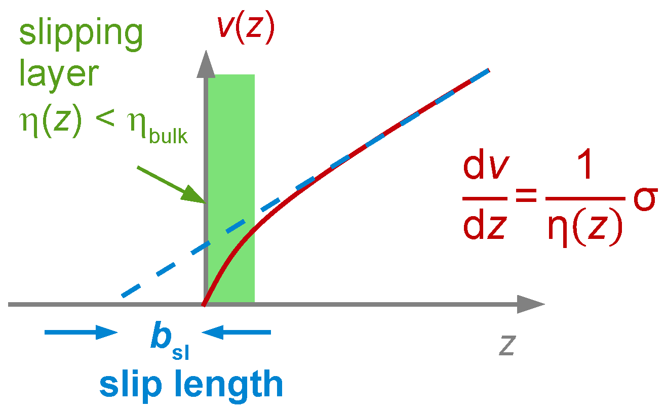
| 4.8. | Slip | 34 |
| 5. | Non-Planar Samples | 35 |
| 5.1. | Point Contacts with Large Objects Clamped in Space by Inertia | 35 |
| 5.2. | Large Amplitudes, Partial Slip | 36 |
| 5.3. | Structured Samples, Numerical Calculations | 40 |
| 5.4. | Roughness | 42 |
| 6. | Coupled Resonances | 43 |
| 6.1. | The Sphere with Moderate Mass | 43 |
| 6.2. | Influence of Rotation on the Frequency Shift | 46 |
| 6.3. | Other Types of Coupled Resonances | 49 |
| 7. | Piezoelectric Stiffening | 50 |
| 8. | Beyond the Parallel-Plate Model | 51 |
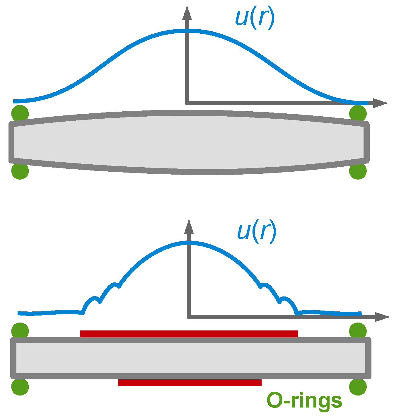
| 8.1. | Energy Trapping, Compressional Waves | 51 |
| 8.2. | Anharmonic Sidebands | 54 |
| 8.3. | Towards 3D-Modelling: The Small-Load Approximation in Tensor Form | 55 |
| 8.4. | The 4-Element Circuit and the Electromechanical Analogy | 58 |
| 8.5. | Amplitude of Oscillation, Effective Area | 60 |
| 8.6. | Modal Mass, Sauerbrey Equation for Plates with Energy Trapping | 61 |
| 9. | Combined Instruments | 62 |
| 9.1. | The Electrochemical QCM (EQCM) | 63 |
| 9.2. | Combination with Optical Reflectometry | 63 |
| References | 71 |
1. Introduction
- Numerous publications discuss the mass uptake of nanoporous and other rigid layers when exposed to a vapor of the analyte [7]. The porous layer takes the role of the receptor. The limit of detection of the QCM easily suffices for sensing building on this principle. (It does not easily suffice for similar sensors, building on adsorption to a planar surface.) These rigid structures swell and soften less than the polymer films, which took a similar role in the past [8]. While the emphasis in these works is on gravimetry, an analysis taking viscoelasticity into account (Equation (46)) will provide for more in-depth information. Also, it will yield a more accurate value for the mass uptake than the Sauerbrey equation.
- The search term “EQCM” returns 137 citations. These are increasingly concerned with an analysis beyond gravimetry. The non-gravimetric effects in this context mostly originate from roughness (Equation (77)), from the viscoelasticity of the double layer (Equation (59)), and from the softness of an active polymer layer (if present, Equation (46)).
- The keyword “QCM-D and brush” returns 37 entries. The brushes often undergo swelling/deswelling transitions or show electroresponsivity. Brushes should be modeled taking viscoelastic effects into account. The shear modulus varies between the bottom and the top, which necessitates the use of a viscoelastic profile (Equation (60)).
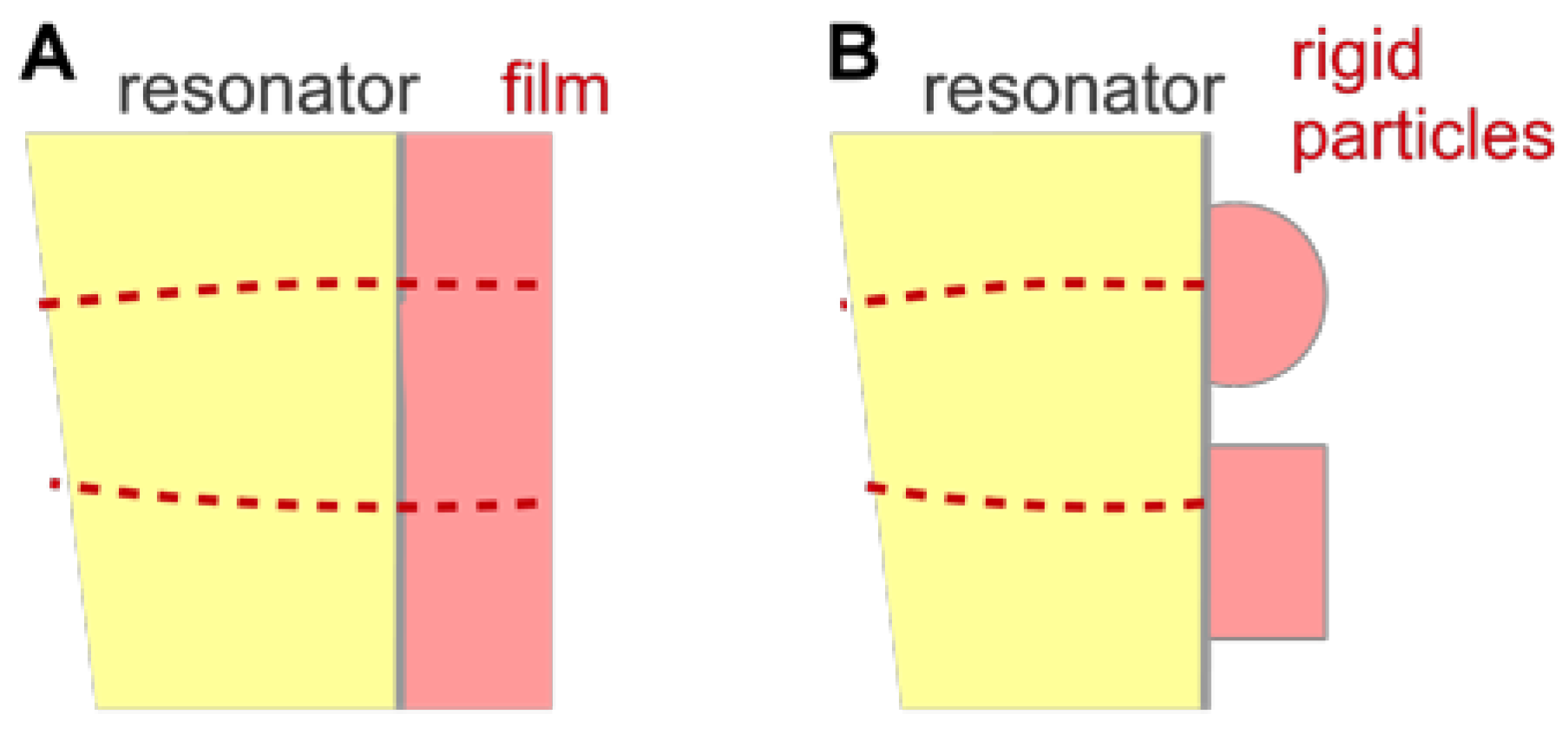
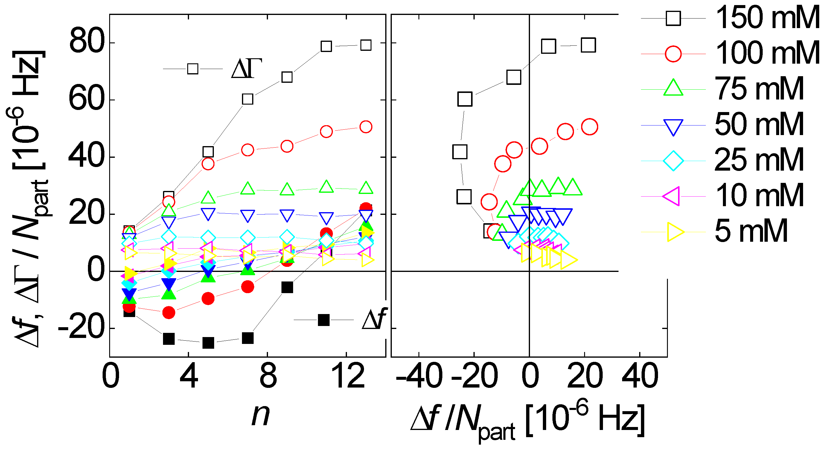
- 114 publications are returned for “QCM and particles”. The interpretation of such QCM data is a topic of ongoing research (Section 6.1 and Section 6.3). For instance, the amount of liquid mass contributing to the gravimetric signal (the “trapped mass”) usually is not known, quantitatively. A few publications explicitly refer to the positive frequency shift induced by sufficiently large particles (Equation (70)).
- 69 publications mention bacteria, which often implies bacterial adsorption (reviewed in [9]). In these cases (and also for cell cultures and biofilms) the shear wave often does not reach to the top of the layer. The QCM then cannot measure the thickness. If such a thick sample is homogeneous in viscoelastic terms, the QCM reports the shear modulus of this medium (Equation (31)). For reviews of applications in the life sciences, in general, see [10,11].
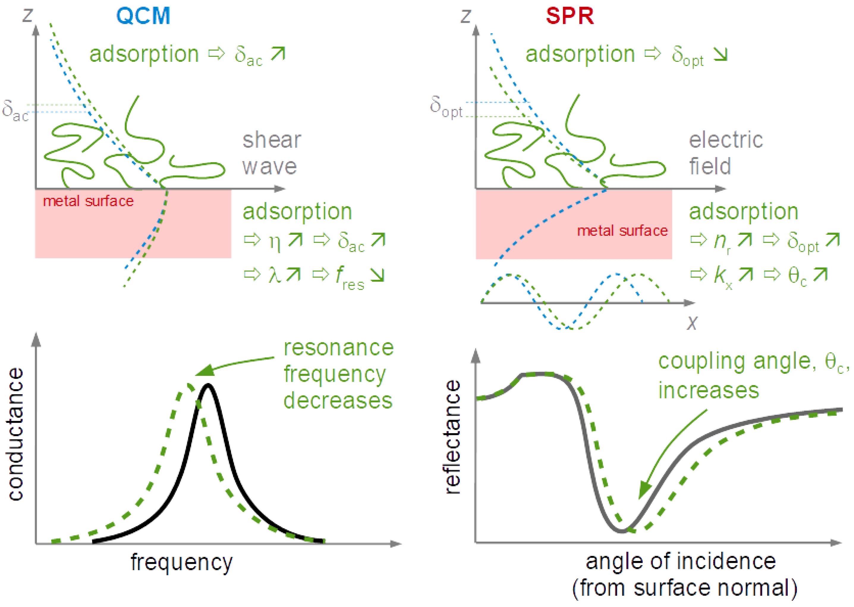
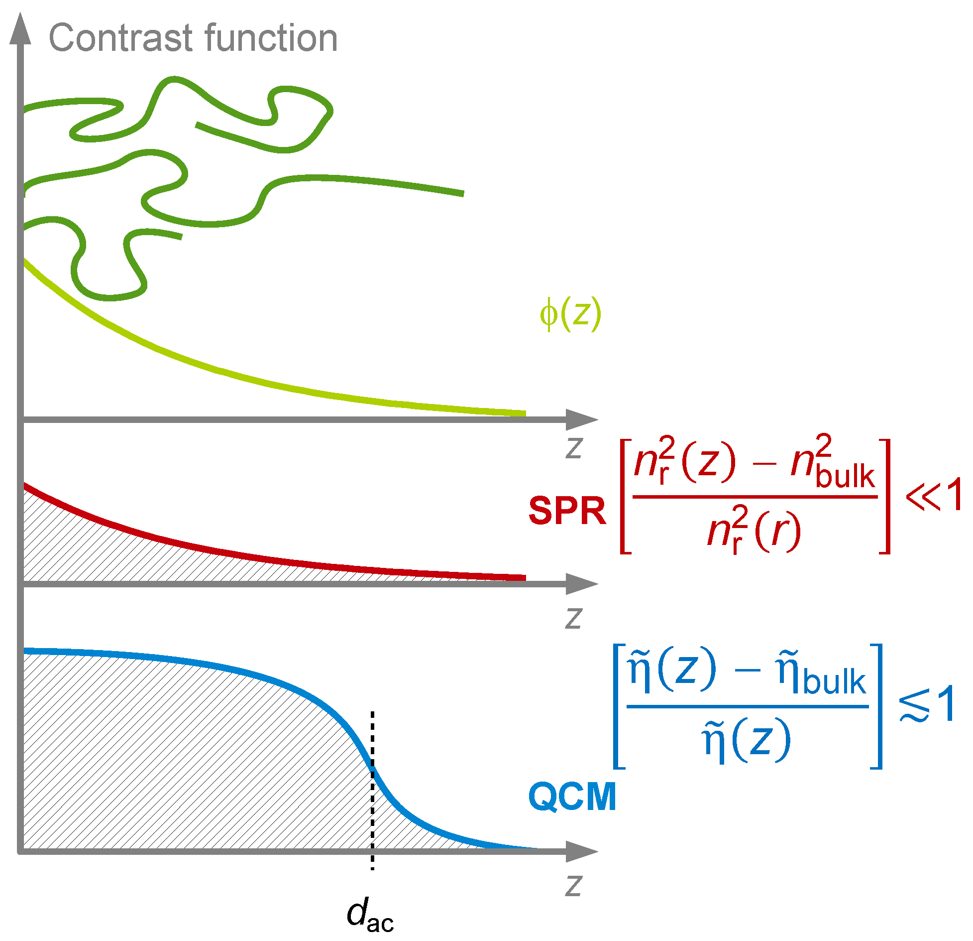
- Interestingly, 247 hits are returned when asking for “QCM and protein”. Protein adsorption is also routinely and successfully probed with optical techniques such as surface plasmon resonance (SPR) spectroscopy. The added information contained in the layer’s viscoelasticity (Equation (52)) is a distinctive advantage of the QCM.
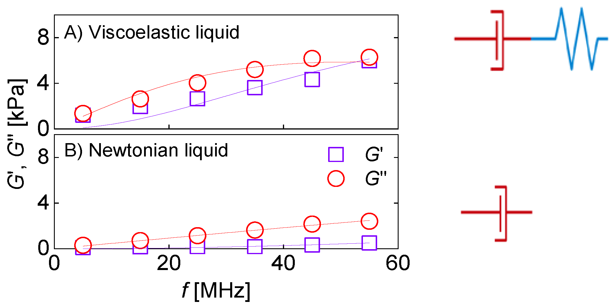
- On the conceptual side, high-frequency rheology on polymers receives considerable attention. Some of these publications are returned when the keyword is “tribology” or “viscoelasticity”. A recent review is contained in [12]. The equations applied for analysis mostly are similar to what is described in Section 4.5.3 and Section 4.6.2. For thick films (microns), Equation (41) is a suitable fit function. Because the frequency shifts are large, temperature effects are irrelevant. For thin films (tens of nanometers), Equation (46) is more suitable than Equation (41). One can hope for data from more than 10 overtones available for analysis. However, the frequency shifts are smaller, which makes the analysis more susceptible to artifacts, for instance caused by changes of temperature.
- Rather few (<10) publications mention large amplitudes and nonlinear behavior. While this is an interesting field in the authors’ opinion, it has not been explored much, yet.
2. Forced Vibrations, Complex Resonance Frequencies
| shear modulus σshear: stress γshear: strain | ||
| viscosity | ||
| shear compliance | ||
| speed of shear sound | ||
| wave number, wave travels towards +z | ||
| wave impedance | ||
| resonance frequency |
3. Techniques of Read-Out
3.1. Oscillator Circuits
3.2. Impedance Analysis
3.3. Ring-Down
3.4. Multi-Frequency Lock-In Amplification
3.5. Fast Measurements, Modulation Experiments
3.6. Noise and Drift
4. The Acoustic Multilayer Formalism and Its Consequences
4.1. Qualitative Data Inspection
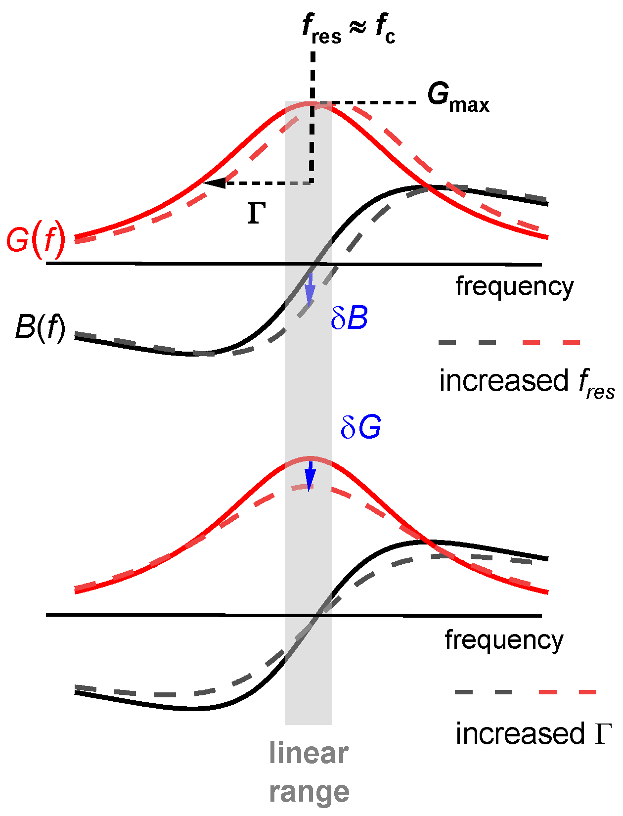
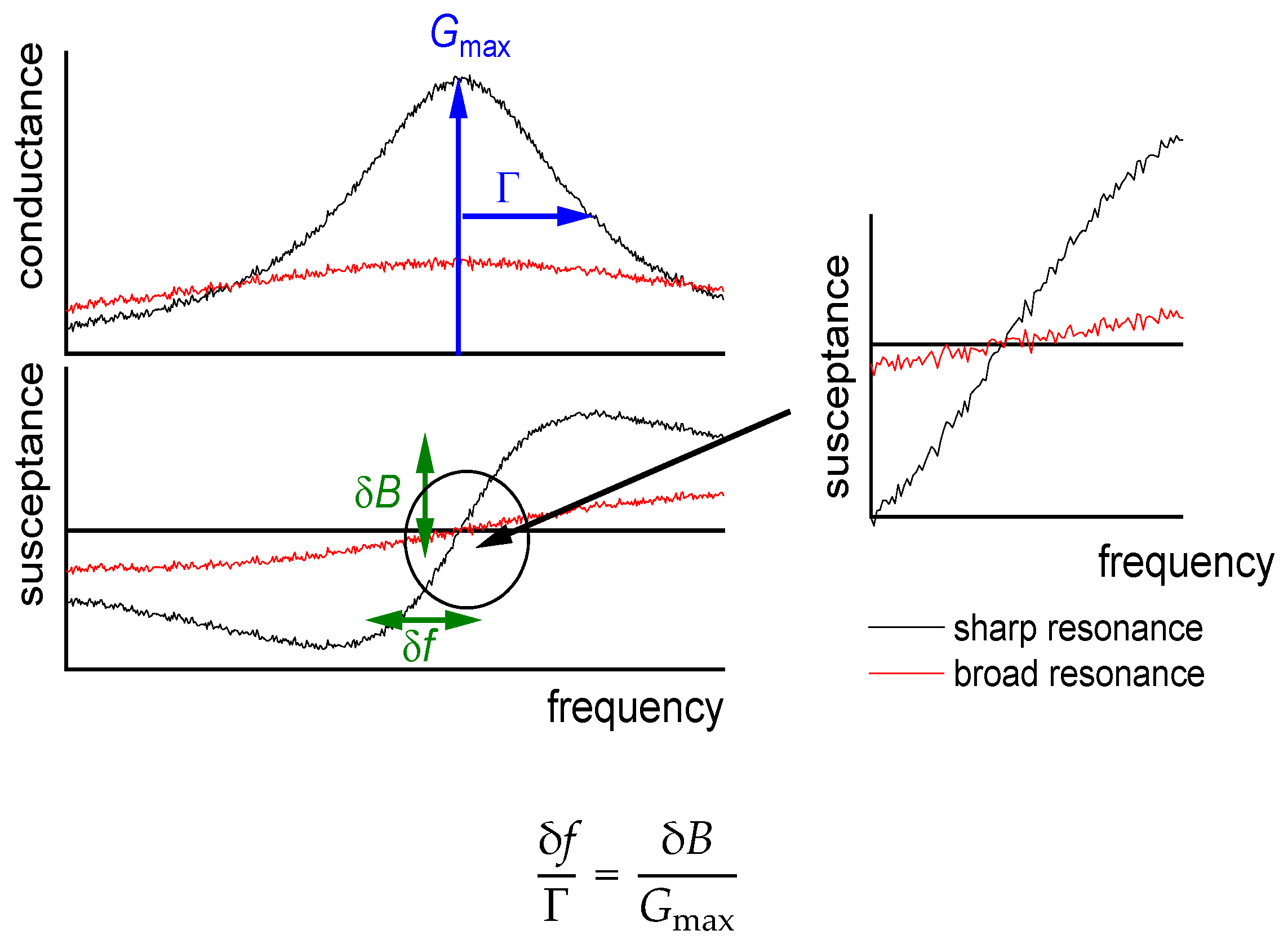
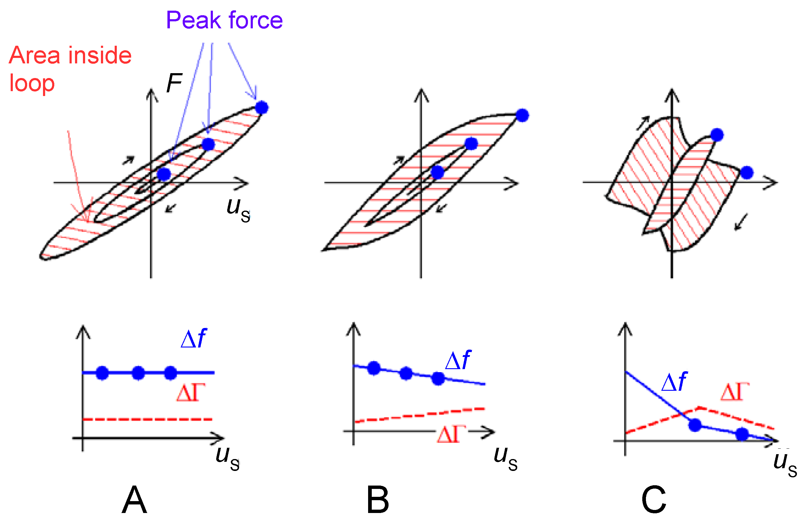
- Is −Δf ΔΓ and is −Δf/n ≈ const.? Did the experiment occur in air? If so, the response is probably dominated by inertia in the sense of the Sauerbrey equation (“inertial loading”). With a density of 1 g/cm3 and 5 MHz crystals, a layer thickness of 1 nm leads to −Δf/n = 5.7 Hz. Did the experiment occur in liquid? If so, the response is probably dominated by the formation of a thin layer. However, −Δf/n may be smaller than 5.7 Hz per nanometer in case the film is soft (Equation (52)).
- Is −Δf ≈ ΔΓ, is −Δf/n1/2 ≈ const., and was the resonator immersed in a liquid? If so, the response is probably dominated by changes in viscosity (Equation (29), “viscous loading”). With 5 MHz crystals, −Δf/n1/2 = 716 Hz corresponds to a viscosity of 1 mPa s (slightly more than the viscosity of water).
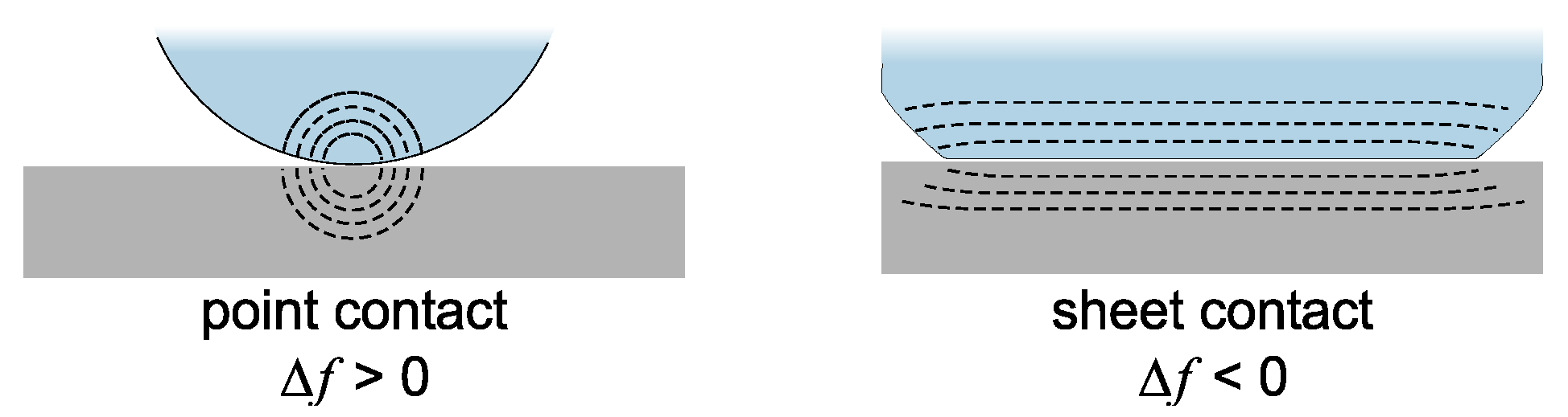
- Is Δf > 0 and is Δf·n ≈ const.? If so, the response may be dominated by point contacts (“elastic loading”, Section 5.1).
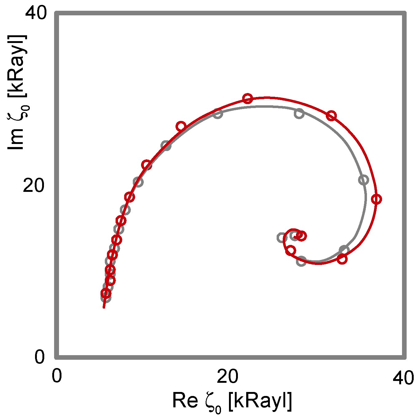
- Do Δf and ΔΓ show unexpected patterns? If plots of ΔΓ versus Δf show circles or spirals, the data may originate from a coupled resonance (Equation (79), Section 6).
4.2. The Small-Load Approximation in 1D (Parallel-Plate Model)
- –
- linearizing the tangent as
- –
- evaluating the load impedance at the frequency of the unloaded crystal, rather than the resonance frequency in the presence of the load.
4.3. Inertial Loading
4.4. Semi-Infinite Viscoelastic Media
4.5. Films in Air
- –
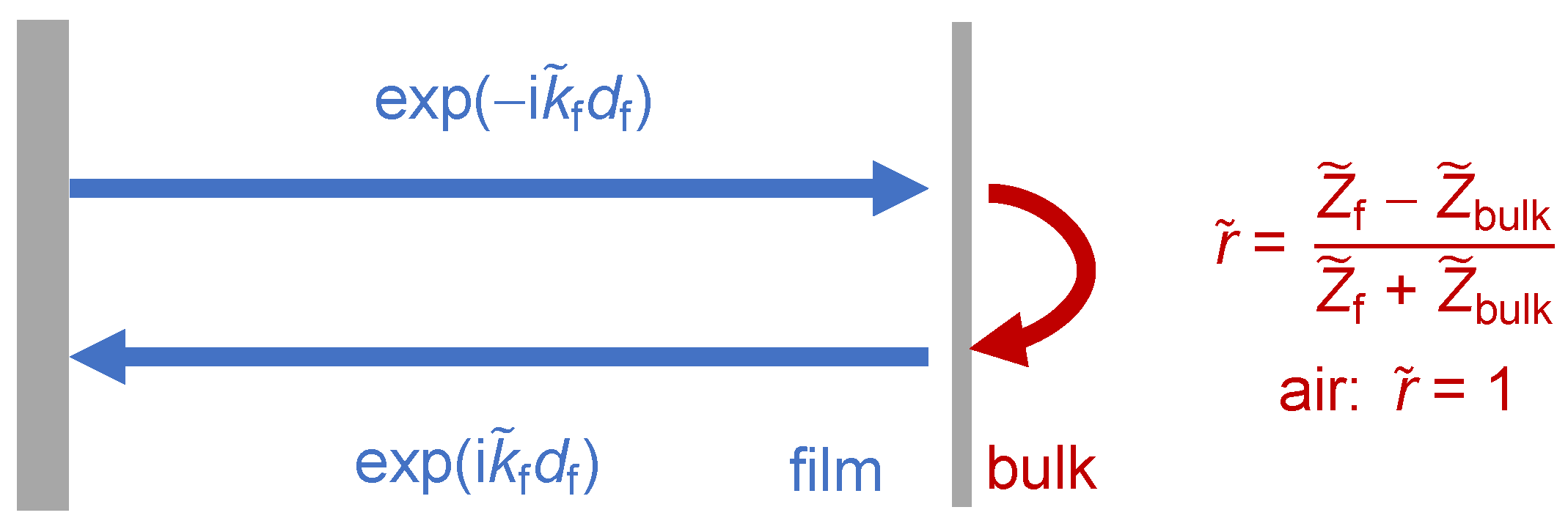
- When an optical wave hits an interface at normal incidence, the reflectivity is . While one might think so, the refractive index, nr, is not strictly the same as the impedance of the optical wave, but it is related to this impedance.
- –
- Upon a central elastic collision of two spheres, the velocity of the first sphere after collision is = . The mass takes the role, which the impedance has for waves.
4.5.1. Very Thin Films (Sauerbrey Limit)
4.5.2. Infinite Thickness
4.5.3. Thin Viscoelastic Films
4.5.4. The Film Resonance
4.6. Layers Adsorbed from a Liquid Phase
4.6.1. General
4.6.2. Thin Adsorbates
- For the thin film in air, the Sauerbrey mass is larger than the true mass. It is smaller for the thin film in a liquid (because of the missing-mass effect).
- The viscoelastic correction scales as n2 in air, while it scales as n in liquids (constant compliance assumed).
- In both cases, and are the coefficients to the viscoelastic correction. In air, enters the correction for −Δf/n, while enters the correction for ΔΓ/n. The roles of and are reversed in liquids.
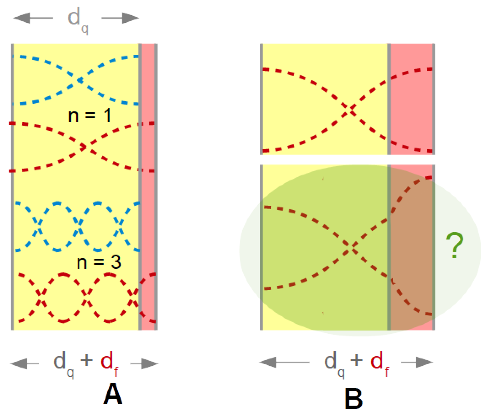
- In air, the viscoelastic correction scales as the square of the film’s mass because the film shears under its own inertia. Viscoelastic effects are only seen for films with a thickness of at least a few tens of nanometers. The film in a liquid is clamped from the other side. Viscoelastic effects are seen even for layers with a thickness corresponding to a few molecules.
4.6.3. Thick Layers
4.7. Viscoelastic Dispersion and High-Frequency Rheology
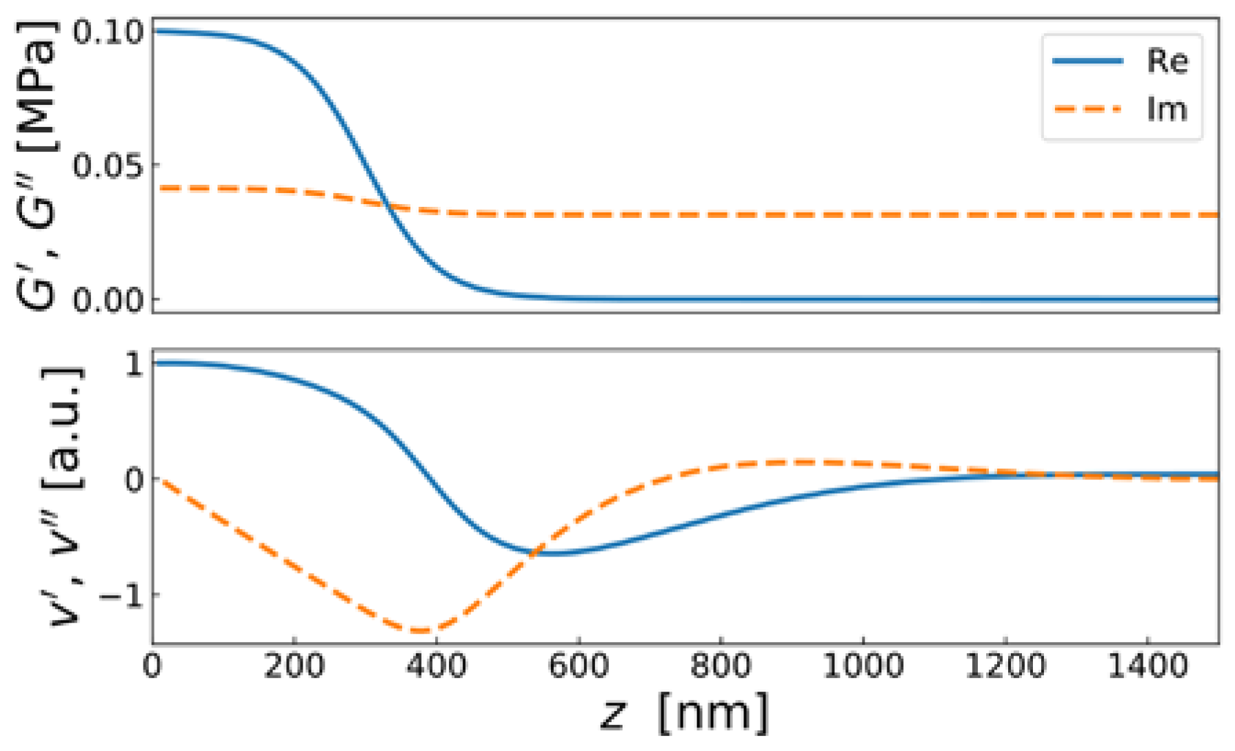
4.8. Slip
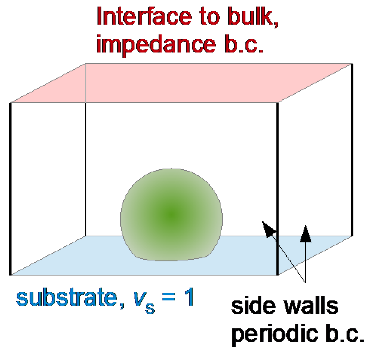
- Nanobubbles constitute a sample with lateral structure, while Equation (68) assumes lateral homogeneity.
- This discussion ignores the surface energy of air-water interfaces (between the nanobubbles and the bulk liquid). Surface tension does play a role on the nanoscale. Surface tension turns nanobubbles into stiff objects [114,115]. (For macroscopic droplets or bubbles, the surface energy does not affect the resonance frequency because the associated oscillatory capillary pressure is small compared to the viscous stress.)
5. Non-Planar Samples
5.1. Point Contacts with Large Objects Clamped in Space by Inertia
5.2. Large Amplitudes, Partial Slip
- Unbinding of virus particles at high amplitudes was studied in [124].
- Adsorption was prevented at high amplitudes in [125] and other publications by the same group.
- Cell adhesion as a function of amplitude was studied in [126]. Cell adhesion was delayed by high amplitudes, but cells, which had already adhered, did not detach when shaken vigorously.
- High amplitudes can induce steady streaming, as shown in [127]. More generally, the Reynolds number at high amplitude can be large enough to let the nonlinear term in the Navier-Stokes equation (of the form ) be significant. This term can cause an oscillatory Bernoulli pressure. There may be a net attractive force onto colloidal particles, mediated by a high-frequency version of the Magnus force [128].
5.3. Structured Samples, Numerical Calculations
5.4. Roughness
6. Coupled Resonances
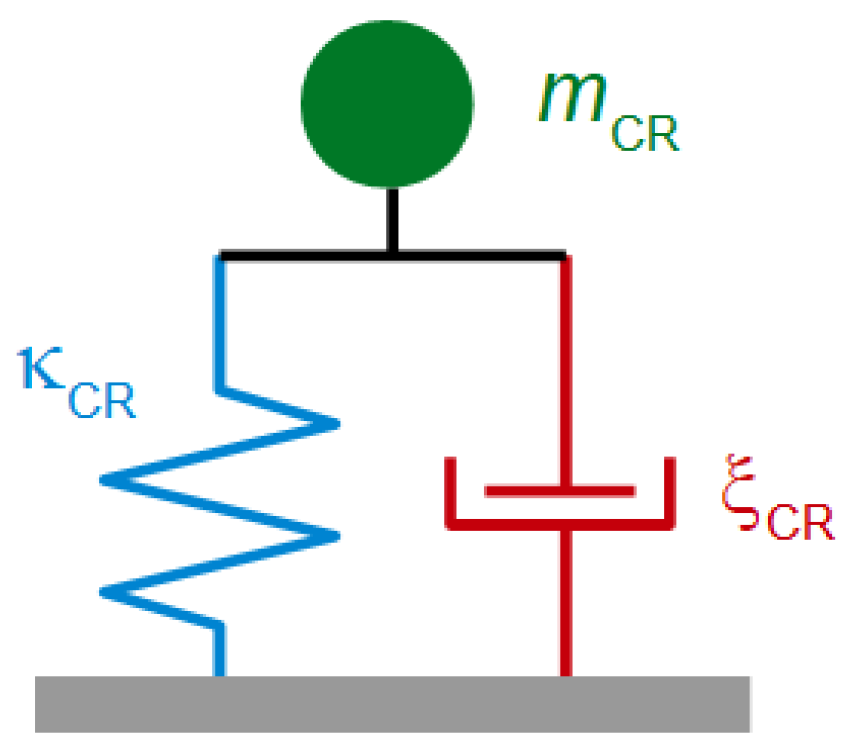
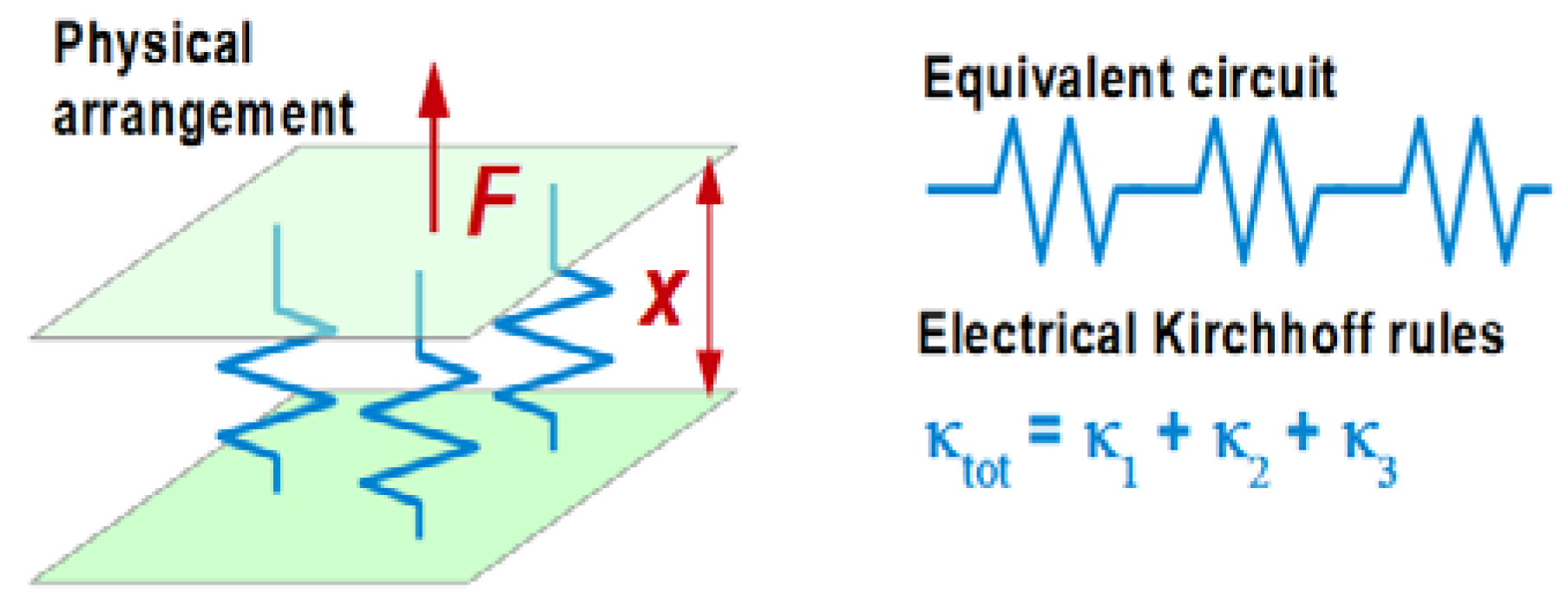
6.1. The Sphere with Moderate Mass
| Electrical | Mechanical | ||
| Voltage U | Force F | ||
| Current I | Velocity v | ||
Resistor | Dashpot | ||
Capacitor | Spring | ||
Inductor | Mass | ||
| Elements in parallel | Elements in parallel | ||
| Elements in series | Elements in series | ||
| Ground | U = 0 | Open end | F = 0 |
| Open end | I = 0 | Wall | V = 0 |
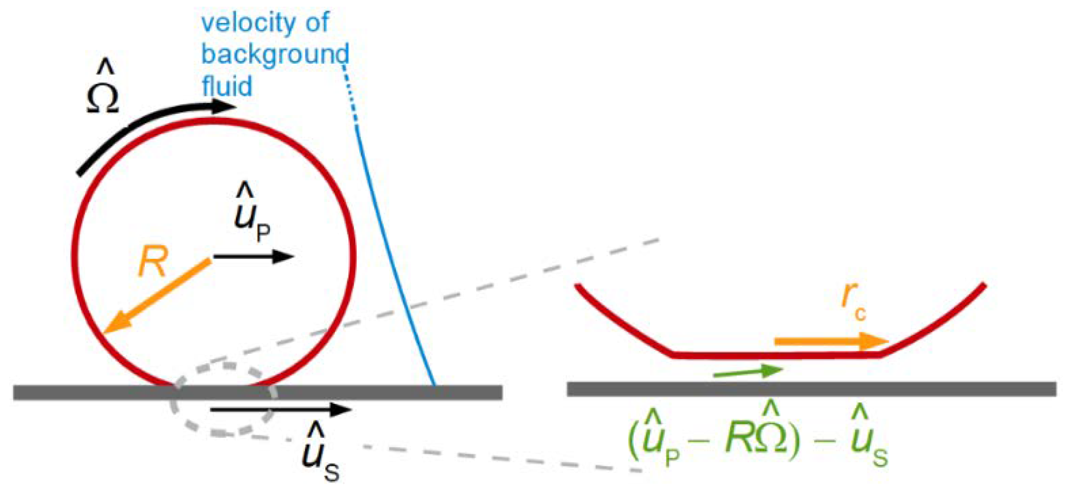
6.2. Influence of Rotation on the Frequency Shift
6.3. Other Types of Coupled Resonances
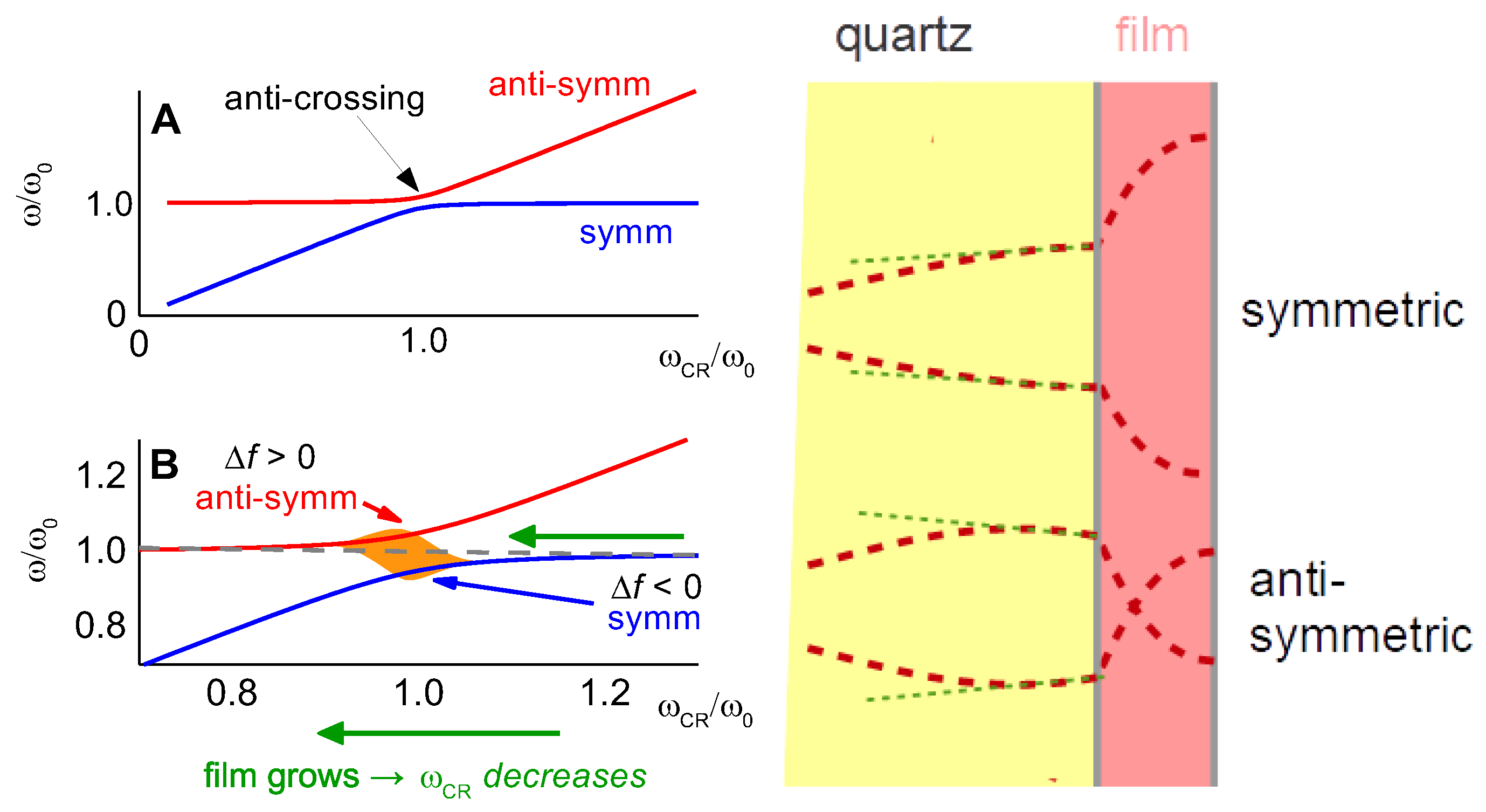
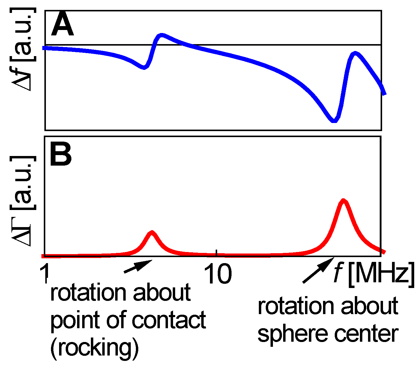
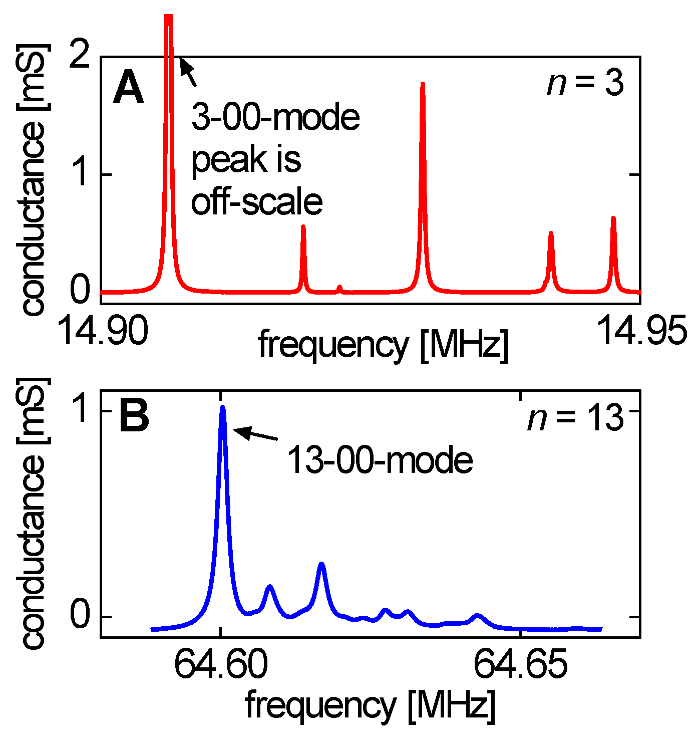
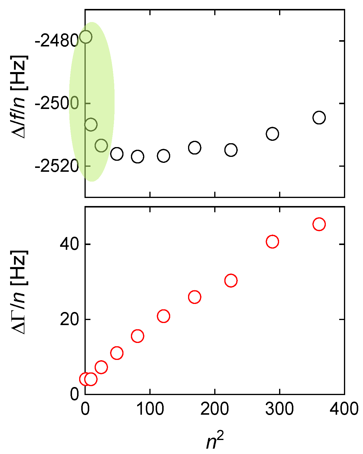
- Standing compressional waves (Section 8.1) give rise to coupled resonances, when the distance to the opposite cell wall is an integer multiple of half the wavelength. At these distances, the compressional wave is a standing wave and the damping is large. This phenomenon can be exploited to check for the magnitude of compressional wave effects. The experiment is simple. One lets the water level in an open cell slowly decrease by evaporation overnight. Figure 7 in [172] shows data of this kind. In this example, the compressional wave effects were much stronger on the fundamental than at 15 MHz. This is a general rule and one of the reasons, why data from the fundamental often are discarded from the analysis.
- The vibration of interest may couple to other modes of vibration of the crystal, where the exact mechanism of coupling is unclear and where even the nature of the other mode is unclear. These so-called “activity dips”, which sometimes occur when ramping temperature up or down, can be a problem in time and frequency control [173]. An activity dip lets the bandwidth increase at a certain temperature and lets the frequency go through a corresponding antisymmetric pattern. Activity dips are not discussed further here, even though they are occasionally seen in sensing, mostly during temperature sweeps.
7. Piezoelectric Stiffening
8. Beyond the Parallel-Plate Model
8.1. Energy Trapping, Compressional Waves
8.2. Anharmonic Sidebands
8.3. Towards 3D-Modelling: The Small-Load Approximation in Tensor Form
- Piezoelectric stiffening is not included. That can be done (in tensor form). It is simply a matter of not letting oneself be intimidated by large equation systems.
- Some perturbations may actually be large perturbations. Among these are the compressional waves, because the plate’s stiffness under bending (not shear) may be too small to let the normal pressure exerted by compressional waves be a small perturbation [127].
- The above mathematics covers the 1st-order perturbation, only. 3rd-order perturbation is sometimes needed (Box 2).
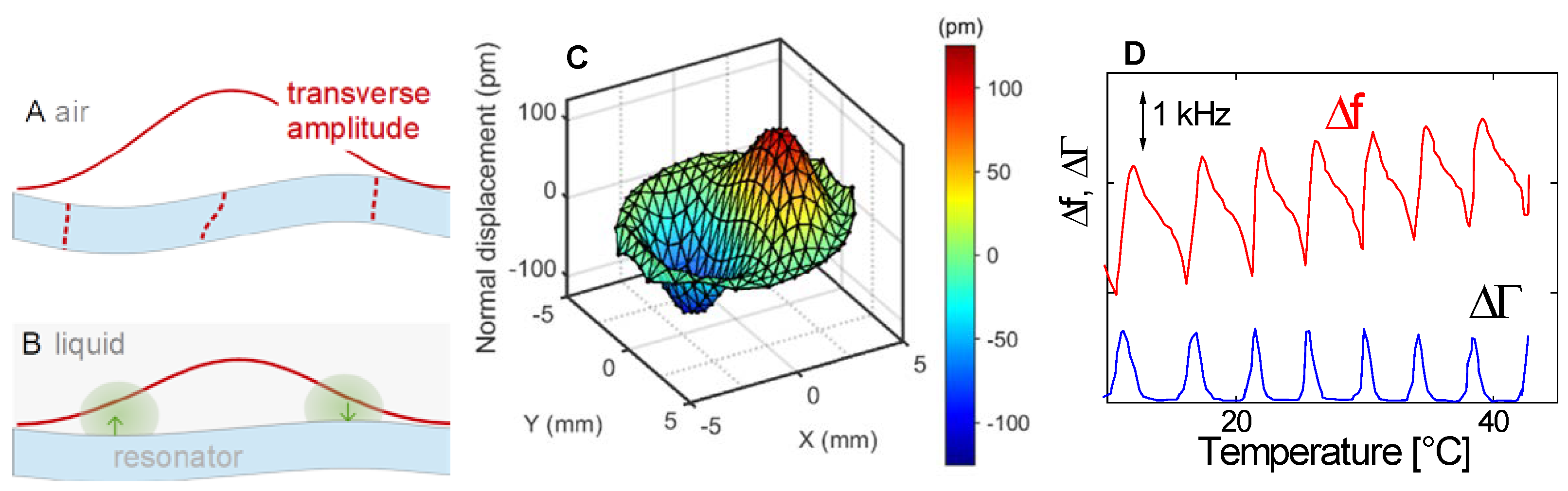
- Calculating the vibration pattern of the unloaded crystal with electrodes is a challenge. If such a calculation is not feasible, the mode of vibration can still be determined experimentally with laser Doppler vibrometry (LDV, Figure 39C).
- It clarifies, why the statistical weight in area averaging in Equation (26) is the square of the local amplitude of oscillation.
- It explains why the Sauerbrey relation is slightly incorrect on the low overtones, even for rigid films in dry environments. The problem is linked to the modal mass (Section 8.6).
8.4. The 4-Element Circuit and the Electromechanical Analogy
8.5. Amplitude of Oscillation, Effective Area
8.6. Modal Mass, Sauerbrey Equation for Plates with Energy Trapping
9. Combined Instruments
- When combining a QCM with an AFM [201], the QCM does not usually respond to the contact with the AFM tip because the contact is too small. That can be understood from Equation (70) together from the Mindlin result for the transverse contact stiffness, which is = 2G* with G* an effective modulus and the contact radius [117] (see Section 5). Inserting values (G* ≈ 10 GPa, ≈ 5 nm) leads to a frequency shift below 0.1 Hz (at 5 MHz). An AFM tip tapping onto the resonator amounts to a nanoscopic object perturbing the motion of a macroscopic object. It does so, in principle, but the effects usually disappear in the noise. In the reverse direction (the QCM perturbing the motion of the tip), there is a strong influence [202]. However, experiments of this kind can also be done with any other actuator. Nanoscale dynamical-mechanical studies based on an AFM tip in contact with a vibrating substrate are commonplace ([203] and others).
- In-situ combination with dielectric spectroscopy [204,205,206,207] or electrical cell-substrate impedance spectroscopy (ECIS [208]) is possible. A difficulty arises, when the sample requires an oxidic substrate, such as SiOx, because the commercially available SiOx coatings may be too thick. The electric field then does not reach to the sample. More technically, the coating’s capacitance, CSiOx, is so small, that its impedance dominates the sample’s overall electrical impedance. The properties of the sample are then masked by the term 1/(iωCSiOx). Thin dielectric coatings are needed.
9.1. The Electrochemical QCM (EQCM)
9.2. Combination with Optical Reflectometry
Author Contributions
Funding
Institutional Review Board Statement
Informed Consent Statement
Data Availability Statement
Acknowledgments
Conflicts of Interest
Appendix A. Summary of Essential Equations
| Small-load approximation | |
| Gordon-Kanazawa equation, semi-infinite viscoelastic medium | |
| Sauerbrey equation, rigid sample | |
| Viscoelastic film in air | |
| Thin film in air | |
| Viscoelastic film in liquid | |
| Thin film in liquid | |
| Thin adsorbate in liquid | |
| Point contacts | |
| Time averaging, large amplitudes, nonlinear response | |
| Small-load approximation in tensor form | |
| Piezoelectric stiffening |
Appendix B. Glossary of Variables and Relations
| Variable | Definition | ||
| ~ | Tilde: a complex parameter | ||
| ^ | Hat: a complex amplitude | ||
| Effective area of the resonator | (A1) | ||
| Resonator’s electrical capacitance (parallel capacitance) | (A2) | ||
| Motional capacitance | (A3) | ||
| D | Dissipation factor | (A4) | |
| Shear modulus | (A5) | ||
| Shear modulus of AT-cut quartz | ≈ 29 × 109 Pa | ||
| Shear compliance | (A6) | ||
| Motional inductance | (A7) | ||
| Q | Quality factor | (A8) | |
| R1 | Motional resistance, the inverse of Gmax (Equation (13)) | ||
| Shear-wave impedance | (A9) | ||
| Load impedance | (A10) | ||
| Shear-wave impedance of AT-cut quartz | = 8.8 × 10⁶ kg m−2 s−1 | ||
| Speed of shear sound | |||
| Piezoelectric strain coefficient of AT-cut quartz | = 3.1 × 10⁻¹² m/V | ||
| Piezoelectric stress coefficient of AT-cut quartz | = 9.65 × 10⁻² C/m2 | ||
| Thickness of film and resonator | |||
| Wave vector in the film, the resonator plate, and the bulk | (A11) | ||
| Electromechanical coupling coefficient | (A12) | ||
| A frequency in the center of the QCM’s frequency range (Section 4.7) | |||
| Resonance frequency in reference state | |||
| Resonance frequency | |||
| Fundamental frequency | |||
| Mass per unit area of the film and the resonator plate | (A13) | ||
| Effective mass of a resonator | (A14) | ||
| n | Overtone order | ||
| Number of particles in contact with the resonator | |||
| Refractive index | |||
| Displacement, amplitude of displacement (^) subscript S: at the surface | (A15) | ||
| , | Velocity, amplitude of velocity (^) | (A16) | |
| Power law exponents, Section 4.7 | (A17) | ||
| Viscosity | (A18) | ||
| Γ | Imaginary part of resonance frequency, half-band half width | ||
| Load impedance in electrical units (in older publications) | (A19) | ||
| Dielectric constant of AT-cut quartz | = 4.54 | ||
| Effective spring constant | (A20) | ||
| Density of α-quartz | = 2.65 × 10³ kg/m3 | ||
| , | Tangential stress, amplitude thereof | ||
| Effective drag coefficient |
Appendix C. Python Code
Appendix C.1. Calculation of Δf + iΔΓ Resulting from a Continuous Viscoelastic Profile
- The algorithm solve_ivp from scipy requires the 2nd-order differential equation from Equation (64) to be turned into a system of two 1st-order equations. This is achieved by defining the function . The 1st-order equations are:
- One choses an “initial” condition at large z and integrates backwards. In this way, it is ensured that the solution decays to zero as z∞. The initial condition consists of values for the velocity and the velocity gradient. The velocity can take any value. It later cancels during normalization. The velocity gradient is the velocity multiplied by i where is the wave number in the bulk liquid.
Appendix C.2. Calculation of Δf + iΔΓ for a Film in Air, Starting from the Lu-Lewis Equation
Appendix C.3. Fit of a Box Profile to Experimental Data
Appendix D. Justification of a Complex in the Lu-Lewis Equation
References
- Steinem, C.; Janshoff, A. Piezoeletric Sensors; Springer: Berlin/Heidelberg, Germany, 2007. [Google Scholar] [CrossRef]
- Bunde, R.L.; Jarvi, E.J.; Rosentreter, J.J. Piezoelectric quartz crystal biosensors. Talanta 1998, 46, 1223–1236. [Google Scholar] [CrossRef]
- Marx, K.A. Quartz crystal microbalance: A useful tool for studying thin polymer films and complex biomolecular systems at the solution-surface interface. Biomacromolecules 2003, 4, 1099–1120. [Google Scholar] [CrossRef] [Green Version]
- Rickert, J.; Brecht, A.; Göpel, W. Quartz crystal microbalances for quantitative biosensing and characterizing protein multilayers. Biosens. Bioelectron. 1997, 12, 567–575. [Google Scholar] [CrossRef]
- Johannsmann, D. The Quartz Crystal Microbalance in Soft Matter Research: Fundamentals and Modeling; Springer: Cham, Switzerland, 2015. [Google Scholar] [CrossRef]
- Thompson, M.; Kipling, A.L.; Duncanhewitt, W.C.; Rajakovic, L.V.; Cavicvlasak, B.A. Thickness-Shear-Mode Acoustic-Wave Sensors in the Liquid-Phase—A Review. Analyst 1991, 116, 881–890. [Google Scholar] [CrossRef]
- Torad, N.; Zhang, S.; Amer, W.; Ayad, M.; Kim, M.; Kim, J.; Ding, B.; Zhang, X.; Kimura, T.; Yamauchi, Y. Advanced Nanoporous Material-Based QCM Devices: A New Horizon of Interfacial Mass Sensing Technology. Adv. Mater. Interfaces 2019, 6, 1900849. [Google Scholar] [CrossRef]
- Grate, J.W. Acoustic wave microsensor arrays for vapor sensing. Chem. Rev. 2000, 100, 2627–2647. [Google Scholar] [CrossRef] [PubMed]
- Alexander, T.E.; Lozeau, L.D.; Camesano, T.A. QCM-D characterization of time-dependence of bacterial adhesion. Cell Surf. 2019, 5, 100024. [Google Scholar] [CrossRef]
- Huang, R.; Yi, R.; Tang, Y. Probing the interactions of organic molecules, nanomaterials, and microbes with solid surfaces using quartz crystal microbalances: Methodology, advantages, and limitations. Environ. Sci. Process. Impacts 2017, 19, 793–811. [Google Scholar] [CrossRef]
- Kuchmenko, T.; Lvova, L. A perspective on recent advances in piezoelectric chemical sensors for environmental monitoring and foodstuffs analysis. Chemosensors 2019, 7, 39. [Google Scholar] [CrossRef] [Green Version]
- Delgado, D.E.; Sturdy, L.F.; Burkhart, C.W.; Shull, K.R. Validation of quartz crystal rheometry in the megahertz frequency regime. J. Polym. Sci. B-Polym. Phys. 2019, 57, 1246–1254. [Google Scholar] [CrossRef]
- Sauerbrey, G. Verwendung von Schwingquarzen zur Wägung Dünner Schichten und zur Mikrowägung. Z. Phys. 1959, 155, 206–222. [Google Scholar] [CrossRef]
- The Sound of Bells. Available online: http://www.hibberts.co.uk/tuning.htm (accessed on 10 May 2021).
- Surface Acoustic Wave Sensors (SAWS): Design for Application. Available online: http://www.jaredkirschner.com/uploads/9/6/1/0/9610588/saws.pdf (accessed on 10 May 2021).
- Homola, J.; Yee, S.S.; Gauglitz, G. Surface plasmon resonance sensors: Review. Sens. Actuators B Chem. 1999, 54, 3–15. [Google Scholar] [CrossRef]
- Lu, C.; Czanderna, A.W. Applications of Piezoelectric Quartz Crystal Microbalances; Elsevier: Amsterdam, The Netherlands, 1984. [Google Scholar] [CrossRef]
- Nomura, T.; Okuhara, M. Frequency-Shifts of Piezoelectric Quartz Crystals Immersed in Organic Liquids. Anal. Chim. Acta 1982, 142, 281–284. [Google Scholar] [CrossRef]
- Nomura, T.; Hattori, O. Determination of Micromolar Concentrations of Cyanide in Solution with a Piezoelectric Detector. Anal. Chim. Acta 1980, 115, 323–326. [Google Scholar] [CrossRef]
- Bruckenstein, S.; Shay, M. Experimental Aspects of Use of the Quartz Crystal Microbalance in Solution. Electrochim. Acta 1985, 30, 1295–1300. [Google Scholar] [CrossRef]
- Jones, J.L.; Mieure, J.P. A Piezoelectric Transducer for Determination of Metals at Micromolar Level. Anal. Chem. 1969, 41, 484–490. [Google Scholar] [CrossRef]
- Martin, S.J.; Granstaff, V.E.; Frye, G.C. Characterization of a Quartz Crystal Microbalance with Simultaneous Mass and Liquid Loading. Anal. Chem. 1991, 63, 2272–2281. [Google Scholar] [CrossRef]
- Kanazawa, K.K.; Gordon, J.G. Frequency of a Quartz Microbalance in Contact with Liquid. Anal. Chem. 1985, 57, 1770–1771. [Google Scholar] [CrossRef]
- Stockbridge, C.D. Effects of Gas Pressure on Quartz-Crystal Microbalances. In Vacuum Microbalance Techniques; Plenum Press: New York, NY, USA, 1966; Volume 5, pp. 147–178. [Google Scholar]
- Mason, W.P. Piezoelectric Crystals and their Applications to Ultrasonics; Van Nostrand: Princeton, NJ, USA, 1948. [Google Scholar]
- Reinisch, L.; Kaiser, R.D.; Krim, J. Measurement of Protein Hydration Shells Using a Quartz Microbalance. Phys. Rev. Lett. 1989, 63, 1743–1746. [Google Scholar] [CrossRef] [Green Version]
- Beck, R.; Pittermann, U.; Weil, K.G. Impedance analysis of quartz oscillators, contacted on one side with a liquid. Ber. Bunsen-Ges. Phys. Chem. 1988, 92, 1363–1368. [Google Scholar] [CrossRef]
- Buttry, D.A.; Ward, M.D. Measurement of Interfacial Processes at Electrode Surfaces with the Electrochemical Quartz Crystal Microbalance. Chem. Rev. 1992, 92, 1355–1379. [Google Scholar] [CrossRef]
- Sittel, K.; Rouse, P.E.; Bailey, E.D. Method for Determining the Viscoelastic Properties of Dilute Polymer Solutions at Audio-Frequencies. J. Appl. Phys. 1954, 25, 1312–1320. [Google Scholar] [CrossRef]
- Rodahl, M.; Hook, F.; Krozer, A.; Brzezinski, P.; Kasemo, B. Quartz-Crystal Microbalance Setup for Frequency and Q-Factor Measurements in Gaseous and Liquid Environments. Rev. Sci. Instrum. 1995, 66, 3924–3930. [Google Scholar] [CrossRef] [Green Version]
- Hirao, M.; Ogi, H.; Fukuoka, H. Resonance Emat System for Acoustoelastic Stress Measurement in Sheet Metals. Rev. Sci. Instrum. 1993, 64, 3198–3205. [Google Scholar] [CrossRef] [Green Version]
- Many of these units build on a design published by Paul Kiciak. Available online: https://www.makarov.ca/vna.htm (accessed on 10 May 2021).
- Eggers, F.; Funck, T. Method for Measurement of Shear-Wave Impedance in the Mhz Region for Liquid Samples of Approximately 1 Ml. J. Phys. E 1987, 20, 523–530. [Google Scholar] [CrossRef]
- Available online: https://en.wikipedia.org/wiki/Grandfather_clock (accessed on 29 April 2021).
- Lucklum, R.; Eichelbaum, F. Interface Circuits for QCM Sensors. In Piezoelectric Sensors; Springer: Berlin/Heidelberg, Germany, 2007; Volume 5, pp. 3–47. [Google Scholar] [CrossRef]
- Arnau, A. A review of interface electronic systems for AT-cut quartz crystal microbalance applications in liquids. Sensors 2008, 8, 370–411. [Google Scholar] [CrossRef] [PubMed] [Green Version]
- Alassi, A.; Benammar, M.; Brett, D. Quartz Crystal Microbalance Electronic Interfacing Systems: A Review. Sensors 2017, 17, 2799. [Google Scholar] [CrossRef] [PubMed] [Green Version]
- Pierce, G.W. Piezoelectric crystal resonators and crystal oscillators applied to the precision calibration of wavemeters. Proc. Am. Acad. Arts Sci. 1923, 59, 81–106. [Google Scholar] [CrossRef]
- OpenQCM NEXT—Quartz Crystal Microbalance with Dissipation Monitoring and Active Thermal Control. Available online: https://openqcm.com/ (accessed on 30 December 2020).
- Quartz Crystal Microbalance QCM200—5 MHz QCM. Available online: https://www.thinksrs.com/products/qcm200.html (accessed on 30 December 2020).
- Leppin, C.; Hampel, S.; Meyer, F.S.; Langhoff, A.; Fittschen, U.E.A.; Johannsmann, D. A Quartz Crystal Microbalance, Which Tracks Four Overtones in Parallel with a Time Resolution of 10 Milliseconds: Application to Inkjet Printing. Sensors 2020, 20, 5915. [Google Scholar] [CrossRef]
- Gileadi, E. Physical Electrochemistry: Fundamentals, Techniques and Applications; Wiley-VCH: Weinheim, Germany, 2011. [Google Scholar]
- Wudy, F.; Multerer, M.; Stock, C.; Schmeer, G.; Gores, H.J. Rapid impedance scanning QCM for electrochemical applications based on miniaturized hardware and high-performance curve fitting. Electrochim. Acta 2008, 53, 6568–6574. [Google Scholar] [CrossRef]
- Pax, M.; Rieger, J.; Eibl, R.H.; Thielemann, C.; Johannsmann, D. Measurements of fast fluctuations of viscoelastic properties with the quartz crystal microbalance. Analyst 2005, 130, 1474–1477. [Google Scholar] [CrossRef]
- Montagut, Y.; Garcia, J.; Jimenez, Y.; March, C.; Montoya, A.; Arnau, A. Frequency-shift vs phase-shift characterization of in-liquid quartz crystal microbalance applications. Rev. Sci. Instrum. 2011, 82. [Google Scholar] [CrossRef]
- Sapper, A.; Wegener, J.; Janshoff, A. Cell motility probed by noise analysis of thickness shear mode resonators. Anal. Chem. 2006, 78, 5184–5191. [Google Scholar] [CrossRef]
- Guha, A.; Sandstrom, N.; Ostanin, V.; van der Wijngaart, W.; Klenerman, D.; Ghosh, S. Simple and ultrafast resonance frequency and dissipation shift measurements using a fixed frequency drive. Sens. Actuators B-Chem. 2018, 281, 960–970. [Google Scholar] [CrossRef]
- Leppin, C.; Peschel, A.; Meyer, F.; Langhoff, A.; Johannsmann, D. Kinetics of Viscoelasticity in the Electric Double Layer Studied by a Fast Electrochemical Quartz Crystal Microbalance (EQCM). Analyst 2021, 146, 2160–2171. [Google Scholar] [CrossRef]
- Vazquez-Uzal, D.; Gabrielli, C.; Perrot, H.; Rodriguez-Pardo, L.; Rose, D.; Sel, O. Frequency/voltage conversion circuit for alternating current electrogravimetry. Electron. Lett. 2013, 49, 1064–1065. [Google Scholar] [CrossRef]
- Rubiola, E. Phase Noise and Frequency Stability in Oscillators; Cambridge University Press: Cambridge, UK, 2010. [Google Scholar] [CrossRef] [Green Version]
- Rodríguez-Pardo, L.; Rodríguez, J.F.; Gabrielli, C.; Perrot, H.; Brendel, R. Sensitivity, Noise, and Resolution in QCM Sensors in Liquid Media. IEEE Sens. J. 2005, 5, 1251. [Google Scholar] [CrossRef]
- Vig, J.R. Introduction to Quartz Frequency Standards. Available online: https://ieee-uffc.org/frequency-control/educational-resources/introduction-to-quartz-frequency-standards-by-john-r-vig/ (accessed on 10 May 2021).
- Heusler, K.E.; Grzegorzewski, A.; Jackel, L.; Pietrucha, J. Measurement of Mass and Surface Stress at One Electrode of a Quartz Oscillator. Ber. Bunsenges Phys. Chem. 1988, 92, 1218–1225. [Google Scholar] [CrossRef]
- Bandey, H.L.; Martin, S.J.; Cernosek, R.W.; Hillman, A.R. Modeling the responses of thickness-shear mode resonators under various loading conditions. Anal. Chem. 1999, 71, 2205–2214. [Google Scholar] [CrossRef] [PubMed]
- Lucklum, R.; Hauptmann, P. Acoustic microsensors-the challenge behind microgravimetry. Anal. Bioanal. Chem. 2006, 384, 667–682. [Google Scholar] [CrossRef]
- Voinova, M.V.; Rodahl, M.; Jonson, M.; Kasemo, B. Viscoelastic acoustic response of layered polymer films at fluid-solid interfaces: Continuum mechanics approach. Phys. Scr. 1999, 59, 391–396. [Google Scholar] [CrossRef] [Green Version]
- Martin, S.J.; Frye, G.C.; Wessendorf, K.O. Sensing Liquid Properties with Thickness-Shear Mode Resonators. Sens. Actuators A 1994, 44, 209–218. [Google Scholar] [CrossRef]
- Bode, B. Entwicklung Eines Quarzviskometers Für Messungen Bei Hohen Drücken; Clausthal University of Technology: Clausthal, Germany, 1984. [Google Scholar]
- Bücking, W.; Du, B.; Turshatov, A.; Konig, A.M.; Reviakine, I.; Bode, B.; Johannsmann, D. Quartz crystal microbalance based on torsional piezoelectric resonators. Rev. Sci. Instrum. 2007, 78, 074903. [Google Scholar] [CrossRef]
- Bergenholtz, J.; Willenbacher, N.; Wagner, N.J.; Morrison, B.; van den Ende, D.; Mellema, J. Colloidal charge determination in concentrated liquid dispersions using torsional resonance oscillation. J. Colloid Interface Sci. 1998, 202, 430–440. [Google Scholar] [CrossRef]
- McSkimin, H.J. Measurement of Dynamic Shear Viscosity and Stiffness of Viscous Liquids by Means of Traveling Torsional Waves. J. Acoust. Soc. Am. 1952, 24, 355–365. [Google Scholar] [CrossRef]
- Competence in Measurement Technology and Fluid Analysis. Available online: https://flucon.de (accessed on 16 May 2020).
- Schermeyer, M.-T.; Sigloch, H.; Bauer, K.C.; Oelschlaeger, C.; Hubbuch, J. Squeeze flow rheometry as a novel tool for the characterization of highly concentrated protein solutions. Biotechnol. Bioeng. 2016, 113, 576–587. [Google Scholar] [CrossRef]
- Pechhold, W.; Mayer, U.; Raju, G.B.; Guillon, O. Piezo rotary and axial vibrator (PRAV) characterization of a fresh coating during its drying. Rheol. Acta 2011, 50, 221–229. [Google Scholar] [CrossRef]
- Hemsel, T.; Stroop, R.; Uribe, D.O.; Wallaschek, J. Resonant vibrating sensors for tactile tissue differentiation. J. Sound Vib. 2007, 308, 441–446. [Google Scholar] [CrossRef]
- Jakoby, B.; Beigelbeck, R.; Keplinger, F.; Lucklum, F.; Niedermayer, A.; Reichel, E.K.; Riesch, C.; Voglhuber-Brunnmaier, T.; Weiss, B. Miniaturized Sensors for the Viscosity and Density of Liquids-Performance and Issues. Ieee Trans. Ultrason. Ferroelectr. Freq. Control 2010, 57, 111–120. [Google Scholar] [CrossRef]
- Saluja, A.; Kalonia, D.S. Measurement of fluid viscosity at microliter volumes using quartz impedance analysis. Aaps Pharm. Sci. Tech. 2004, 5. [Google Scholar] [CrossRef]
- Flanigan, C.M.; Desai, M.; Shull, K.R. Contact mechanics studies with the quartz crystal microbalance. Langmuir 2000, 16, 9825–9829. [Google Scholar] [CrossRef]
- Herrscher, M.; Ziegler, C.; Johannsmann, D. Shifts of frequency and bandwidth of quartz crystal resonators coated with samples of finite lateral size. J. Appl. Phys. 2007, 101, 114909. [Google Scholar] [CrossRef]
- Hartl, J.; Peschel, A.; Johannsmann, D.; Garidel, P. Characterizing protein-protein-interaction in high-concentration monoclonal antibody systems with the quartz crystal microbalance. Phys. Chem. Chem. Phys. 2017, 19, 32698–32707. [Google Scholar] [CrossRef] [Green Version]
- Saluja, A.; Badkar, A.V.; Zeng, D.L.; Nema, S.; Kalonia, D.S. Application of high-frequency rheology measurements for analyzing protein-protein interactions in high protein concentration solutions using a model monoclonal antibody (IgG(2)). J. Pharm. Sci. 2006, 95, 1967–1983. [Google Scholar] [CrossRef] [PubMed]
- Valtorta, D.; Mazza, E. Measurement of rheological properties of soft biological tissue with a novel torsional resonator device. Rheol. Acta 2006, 45, 677–692. [Google Scholar] [CrossRef] [Green Version]
- Kaatze, U.; Hushcha, T.O.; Eggers, F. Ultrasonic broadband spectrometry of liquids: A research tool in pure and applied chemistry and chemical physics. J. Solut. Chem. 2000, 29, 299–368. [Google Scholar] [CrossRef]
- Mason, W.P.; Baker, W.O.; McSkimin, H.J.; Heiss, J.H. Measurement of Shear Elasticity and Viscosity of Liquids at Ultrasonic Frequencies. Phys. Rev. 1949, 75, 936–946. [Google Scholar] [CrossRef]
- Alig, I.; Oehler, H.; Lellinger, D.; Tadjbach, S. Monitoring of film formation, curing and ageing of coatings by an ultrasonic reflection method. Prog. Org. Coat. 2007, 58, 200–208. [Google Scholar] [CrossRef]
- Lu, C.S.; Lewis, O. Investigation of Film-Thickness Determination by Oscillating Quartz Resonators with Large Mass Load. J. Appl. Phys. 1972, 43, 4385. [Google Scholar] [CrossRef]
- Benes, E. Improved Quartz Crystal Microbalance Technique. J. Appl. Phys. 1984, 56, 608–626. [Google Scholar] [CrossRef]
- QCM100- Quartz Crystal Microbalance Theory and Calibration. Available online: https://www.thinksrs.com/downloads/pdfs/applicationnotes/QCMTheoryapp.pdf (accessed on 10 May 2021).
- Application Note AUTO-Z1: A Path to Precise Control of Layers Thickness. Available online: https://products.inficon.com/getattachment.axd/?attaName=bde54dd9-1870-447e-ba7a-5f737ecdd43e (accessed on 9 March 2021).
- Petri, J.; Johannsmann, D. Determination of the Shear Modulus of Thin Polymer Films with a Quartz Crystal Microbalance: Application to UV-Curing. Anal. Chem. 2019, 91, 1595–1602. [Google Scholar] [CrossRef] [PubMed]
- Wolff, O.; Seydel, E.; Johannsmann, D. Viscoelastic properties of thin films studied with quartz crystal resonators. Faraday Discuss. 1997, 107, 91–104. [Google Scholar] [CrossRef]
- Johannsmann, D. Derivation of the shear compliance of thin films on quartz resonators from comparison of the frequency shifts on different harmonics: A perturbation analysis. J. Appl. Phys. 2001, 89, 6356–6364. [Google Scholar] [CrossRef]
- Sadman, K.; Wiener, C.G.; Weiss, R.A.; White, C.C.; Shull, K.R.; Vogt, B.D. Quantitative Rheometry of Thin Soft Materials Using the Quartz Crystal Microbalance with Dissipation. Anal. Chem. 2018, 90, 4079–4088. [Google Scholar] [CrossRef] [PubMed]
- Shull, K.R.; Taghon, M.; Wang, Q.F. Investigations of the high-frequency dynamic properties of polymeric systems with quartz crystal resonators. Biointerphases 2020, 15, 12. [Google Scholar] [CrossRef] [Green Version]
- Klein, J. Shear, friction, and lubrication forces between polymer-bearing surfaces. Annu. Rev. Mater. Sci. 1996, 26, 581–612. [Google Scholar] [CrossRef]
- Krim, J.; Solina, D.H.; Chiarello, R. Nanotribology of a Kr Monolayer—A Quartz-Crystal Microbalance Study of Atomic-Scale Friction. Phys. Rev. Lett. 1991, 66, 181–184. [Google Scholar] [CrossRef]
- Krim, J. Friction and energy dissipation mechanisms in adsorbed molecules and molecularly thin films. Adv. Phys. 2012, 61, 155–323. [Google Scholar] [CrossRef]
- Salomaki, M.; Kankare, J. Modeling the growth processes of polyelectrolyte multilayers using a quartz crystal resonator. J. Phys. Chem. B 2007, 111, 8509–8519. [Google Scholar] [CrossRef]
- Johannsmann, D.; Mathauer, K.; Wegner, G.; Knoll, W. Viscoelastic Properties of Thin-Films Probed with a Quartz-Crystal Resonator. Phys. Rev. B 1992, 46, 7808–7815. [Google Scholar] [CrossRef]
- Granstaff, V.E.; Martin, S.J. Characterization of a Thickness-Shear Mode Quartz Resonator with Multiple Nonpiezoelectric Layers. J. Appl. Phys. 1994, 75, 1319–1329. [Google Scholar] [CrossRef] [Green Version]
- Martin, S.J.; Bandey, H.L.; Cernosek, R.W.; Hillman, A.R.; Brown, M.J. Equivalent-circuit model for the thickness-shear mode resonator with a viscoelastic film near film resonance. Anal. Chem. 2000, 72, 141–149. [Google Scholar] [CrossRef] [PubMed] [Green Version]
- Thurston, R.N. Piezoelectrically excited vibrations. In Mechanics of Solids; Truesdell, C., Ed.; Springer: Berlin/Heidelberg, Germany, 1984; Volume 4, p. 257. [Google Scholar]
- Domack, A.; Prucker, O.; Ruhe, J.; Johannsmann, D. Swelling of a polymer brush probed with a quartz crystal resonator. Phys. Rev. E 1997, 56, 680–689. [Google Scholar] [CrossRef] [Green Version]
- Johannsmann, D. Viscoelastic, mechanical, and dielectric measurements on complex samples with the quartz crystal microbalance. Phys. Chem. Chem. Phys. 2008, 10, 4516–4534. [Google Scholar] [CrossRef] [Green Version]
- Lekner, J. Theory of Reflection of Electromagnetic and Particle Waves; Springer: Berlin/Heidelberg, Germany, 1987. [Google Scholar] [CrossRef]
- Raudino, M.; Giamblanco, N.; Montis, C.; Berti, D.; Marletta, G.; Baglioni, P. Probing the Cleaning of Polymeric Coatings by Nanostructured Fluids: A QCM-D Study. Langmuir 2017, 33, 5675–5684. [Google Scholar] [CrossRef]
- Li, W.X.; Hu, L.; Zhu, J.H.; Li, D.; Luan, Y.F.; Xu, W.W.; Serpe, M.J. Comparison of the Responsivity of Solution-Suspended and Surface-Bound Poly(N-isopropylacrylamide)-Based Microgels for Sensing Applications. ACS Appl. Mater. Interfaces 2017, 9, 26539–26548. [Google Scholar] [CrossRef]
- Gryte, D.M.; Ward, M.D.; Hu, W.S. Real-Time Measurement of Anchorage-Dependent Cell-Adhesion Using a Quartz Crystal Microbalance. Biotechnol. Prog. 1993, 9, 105–108. [Google Scholar] [CrossRef]
- Wegener, J.; Janshoff, A.; Galla, H.J. Cell adhesion monitoring using a quartz crystal microbalance: Comparative analysis of different mammalian cell lines. Eur. Biophys. J. 1998, 28, 26–37. [Google Scholar] [CrossRef] [PubMed]
- Zhou, T.; Marx, K.A.; Warren, M.; Schulze, H.; Braunhut, S.J. The quartz crystal microbalance as a continuous monitoring tool for the study of endothelial cell surface attachment and growth. Biotechnol. Prog. 2000, 16, 268–277. [Google Scholar] [CrossRef] [PubMed]
- Picart, C.; Lavalle, P.; Hubert, P.; Cuisinier, F.J.G.; Decher, G.; Schaaf, P.; Voegel, J.C. Buildup mechanism for poly(L-lysine)/hyaluronic acid films onto a solid surface. Langmuir 2001, 17, 7414–7424. [Google Scholar] [CrossRef]
- Caruso, F.; Rodda, E.; Furlong, D.F.; Niikura, K.; Okahata, Y. Quartz crystal microbalance study of DNA immobilization and hybridization for nucleic acid sensor development. Anal. Chem. 1997, 69, 2043–2049. [Google Scholar] [CrossRef] [PubMed]
- Gabrielli, C.; Keddam, M.; Minouflet, F.; Perrot, H. Ac electrogravimetry contribution to the investigation of the anodic behaviour of iron in sulfuric medium. Electrochim. Acta 1996, 41, 1217–1222. [Google Scholar] [CrossRef]
- Hillman, A.R.; Efimov, I.; Ryder, K.S. Time-scale- and temperature-dependent mechanical properties of viscoelastic poly(3,4-ethylenedioxythlophene) films. J. Am. Chem. Soc. 2005, 127, 16611–16620. [Google Scholar] [CrossRef]
- Johannsmann, D. Viscoelastic analysis of organic thin films on quartz resonators. Macromol Chem. Phys. 1999, 200, 501–516. [Google Scholar] [CrossRef]
- Voinova, M.V.; Jonson, M.; Kasemo, B. ’Missing mass’ effect in biosensor’s QCM applications. Biosens. Bioelectron. 2002, 17, 835–841. [Google Scholar] [CrossRef]
- Du, B.Y.; Johannsmann, D. Operation of the quartz crystal microbalance in liquids: Derivation of the elastic compliance of a film from the ratio of bandwidth shift and frequency shift. Langmuir 2004, 20, 2809–2812. [Google Scholar] [CrossRef] [PubMed]
- Leger, L.; Hervet, H.; Massey, G.; Durliat, E. Wall slip in polymer melts. J. Phys. Condens. Matter 1997, 9, 7719–7740. [Google Scholar] [CrossRef]
- Huang, D.M.; Sendner, C.; Horinek, D.; Netz, R.R.; Bocquet, L. Water Slippage versus Contact Angle: A Quasiuniversal Relationship. Phys. Rev. Lett. 2008, 101, 226101. [Google Scholar] [CrossRef] [Green Version]
- Neto, C.; Evans, D.R.; Bonaccurso, E.; Butt, H.J.; Craig, V.S.J. Boundary slip in Newtonian liquids: A review of experimental studies. Rep. Prog. Phys. 2005, 68, 2859–2897. [Google Scholar] [CrossRef]
- Bocquet, L.; Charlaix, E. Nanofluidics, from bulk to interfaces. Chem. Soc. Rev. 2010, 39, 1073–1095. [Google Scholar] [CrossRef] [Green Version]
- Falk, K.; Sedlmeier, F.; Joly, L.; Netz, R.R.; Bocquet, L. Ultralow Liquid/Solid Friction in Carbon Nanotubes: Comprehensive Theory for Alcohols, Alkanes, OMCTS, and Water. Langmuir 2012, 28, 14261–14272. [Google Scholar] [CrossRef]
- Seddon, J.R.T.; Lohse, D.; Ducker, W.A.; Craig, V.S.J. A Deliberation on Nanobubbles at Surfaces and in Bulk. Chemphyschem 2012, 13, 2179–2187. [Google Scholar] [CrossRef]
- Finger, A.; Johannsmann, D. Hemispherical nanobubbles reduce interfacial slippage in simple liquids. Phys. Chem. Chem. Phys. 2011, 13, 18015–18022. [Google Scholar] [CrossRef] [PubMed] [Green Version]
- Hyväluoma, J.; Kunert, C.; Harting, J. Simulations of slip flow on nanobubble-laden surfaces. J. Phys. Condens. Matter 2011, 23, 184106. [Google Scholar] [CrossRef] [Green Version]
- Dybwad, G.L. A Sensitive New Method for the Determination of Adhesive Bonding between a Particle and a Substrate. J. Appl. Phys. 1985, 58, 2789–2790. [Google Scholar] [CrossRef]
- Popov, V.L. Contact Mechanics and Friction: Physical Principles and Applications; Springer: Berlin/Heidelberg, Germany, 2010. [Google Scholar] [CrossRef]
- D’Amour, J.N.; Stalgren, J.J.R.; Kanazawa, K.K.; Frank, C.W.; Rodahl, M.; Johannsmann, D. Capillary aging of the contacts between glass spheres and a quartz resonator surface. Phys. Rev. Lett. 2006, 96, 058301. [Google Scholar] [CrossRef]
- Vlachová, J.; König, R.; Johannsmann, D. Stiffness of Sphere–Plate Contacts at MHz Frequencies: Dependence on Normal Load, Oscillation Amplitude, and Ambient Medium. Beilstein J. Nanotechnol. 2015, 6, 845–856. [Google Scholar] [CrossRef] [Green Version]
- Benad, J.; Nakano, K.; Popov, V.L.; Popov, M. Active control of friction by transverse oscillations. Friction 2019, 7, 74–85. [Google Scholar] [CrossRef] [Green Version]
- Scherer, V.; Arnold, W.; Bushan, B. Active Friction Control Using Ultrasonic Vibration. In Tribology Issues and Opportunities in MEMS; Bushan, B., Ed.; Springer: Berlin/Heidelberg, Germany, 1997; pp. 463–469. [Google Scholar] [CrossRef]
- Tshiprut, Z.; Filippov, A.E.; Urbakh, M. Tuning diffusion and friction in microscopic contacts by mechanical excitations. Phys. Rev. Lett. 2005, 95. [Google Scholar] [CrossRef]
- Leopoldes, J.; Jia, X. Transverse Shear Oscillator Investigation of Boundary Lubrication in Weakly Adhered Films. Phys. Rev. Lett. 2010, 105, 266101. [Google Scholar] [CrossRef] [Green Version]
- Cooper, M.A.; Dultsev, F.N.; Minson, T.; Ostanin, V.P.; Abell, C.; Klenerman, D. Direct and sensitive detection of a human virus by rupture event scanning. Nat. Biotechnol. 2001, 19, 833–837. [Google Scholar] [CrossRef] [PubMed]
- Edvardsson, M.; Rodahl, M.; Hook, F. Investigation of binding event perturbations caused by elevated QCM-D oscillation amplitude. Analyst 2006, 131, 822–828. [Google Scholar] [CrossRef] [PubMed]
- Heitmann, V.; Wegener, J. Monitoring cell adhesion by piezoresonators: Impact of increasing oscillation amplitudes. Anal. Chem. 2007, 79, 3392–3400. [Google Scholar] [CrossRef]
- König, R.; Langhoff, A.; Johannsmann, D. Steady flows above a quartz crystal resonator driven at elevated amplitude. Phys. Rev. E 2014, 89, 043016. [Google Scholar] [CrossRef] [PubMed]
- Langhoff, A.; Johannsmann, D. Attractive forces on hard and soft colloidal objects located close to the surface of an acoustic-thickness shear resonator. Phys. Rev. E 2013, 88, 013001. [Google Scholar] [CrossRef]
- Patel, M.S.; Yong, Y.K.; Tanaka, M. Drive level dependency in quartz resonators. Int. J. Solids Struct. 2009, 46, 1856–1871. [Google Scholar] [CrossRef] [Green Version]
- Etsion, I. Revisiting the Cattaneo-Mindlin Concept of Interfacial Slip in Tangentially Loaded Compliant Bodies. J. Tribol. 2010, 132. [Google Scholar] [CrossRef] [Green Version]
- Mindlin, R.D.; Deresiewicz, H. Elastic Spheres in Contact under Varying Oblique Forces. J. Appl. Mech. 1953, 20, 327–344. [Google Scholar]
- Johnson, K.L. Contact Mechanics; Cambridge University Press: Cambridge, UK, 1985. [Google Scholar] [CrossRef]
- Baumberger, T.; Caroli, C. Solid friction from stick-slip down to pinning and aging. Adv. Phys. 2006, 55, 279–348. [Google Scholar] [CrossRef]
- Berthier, Y.; Vincent, L.; Godet, M. Fretting Fatigue and Fretting Wear. Tribol. Int. 1989, 22, 235–242. [Google Scholar] [CrossRef]
- Duran, J. Sands, Powders, and Grains: An Introduction to the Physics of Granular Materials; Springer: Berlin/Heidelberg, Germany, 2000. [Google Scholar] [CrossRef]
- Cattaneo, C. Sul contatto di due corpi elastici: Distribuzione locale dei sforzi. Rend. Acad. Natl. Lincei 1938, 27. [Google Scholar] [CrossRef]
- Strogatz, S. Nonlinear Dynamics and Chaos; Addison-Wesley: Boston, MA, USA, 1996. [Google Scholar]
- Holscher, H.; Allers, W.; Schwarz, U.D.; Schwarz, A.; Wiesendanger, R. Determination of tip-sample interaction potentials by dynamic force spectroscopy. Phys. Rev. Lett. 1999, 83, 4780–4783. [Google Scholar] [CrossRef]
- Savkoor, A.R. Dry Adhesive Contact of Elastomers. Ph.D. Thesis, Delft University of Technology, Delft, The Netherlands, 1987. [Google Scholar]
- Leopoldes, J.; Jia, X. Probing viscoelastic properties of a thin polymer film sheared between a beads layer and an ultrasonic resonator. EPL 2009, 88. [Google Scholar] [CrossRef] [Green Version]
- Hanke, S.; Petri, J.; Johannsmann, D. Partial slip in mesoscale contacts: Dependence on contact size. Phys. Rev. E 2013, 88, 032408. [Google Scholar] [CrossRef] [PubMed]
- Borovsky, B.P.; Bouxsein, C.; O’Neill, C.; Sletten, L.R. An Integrated Force Probe and Quartz Crystal Microbalance for High-Speed Microtribology. Tribol. Lett. 2017, 65. [Google Scholar] [CrossRef]
- Roach, P.; Farrar, D.; Perry, C.C. Interpretation of protein adsorption: Surface-induced conformational changes. J. Am. Chem. Soc. 2005, 127, 8168–8173. [Google Scholar] [CrossRef]
- Michna, A.; Pomorska, A.; Nattich-Rak, M.; Wasilewska, M.; Adamczyk, Z. Hydrodynamic Solvation of Poly(amido amine) Dendrimer Monolayers on Silica. J. Phys. Chem. C 2020, 124, 17684–17695. [Google Scholar] [CrossRef]
- Wegener, J.; Janshoff, A.; Steinem, C. The quartz crystal microbalance as a novel means to study cell-substrate interactions in situ. Cell Biochem. Biophys. 2001, 34, 121–151. [Google Scholar] [CrossRef]
- Chen, Q.; Xu, S.M.; Liu, Q.X.; Masliyah, J.; Xu, Z.H. QCM-D study of nanoparticle interactions. Adv. Colloid Interface Sci. 2016, 233, 94–114. [Google Scholar] [CrossRef] [Green Version]
- Olsson, A.L.J.; Quevedo, I.R.; He, D.Q.; Basnet, M.; Tufenkji, N. Using the Quartz Crystal Microbalance with Dissipation Monitoring to Evaluate the Size of Nanoparticles Deposited on Surfaces. ACS Nano 2013, 7, 7833–7843. [Google Scholar] [CrossRef] [Green Version]
- Keller, C.A.; Kasemo, B. Surface specific kinetics of lipid vesicle adsorption measured with a quartz crystal microbalance. Biophys. J. 1998, 75, 1397–1402. [Google Scholar] [CrossRef] [Green Version]
- Cho, N.J.; Frank, C.W.; Kasemo, B.; Hook, F. Quartz crystal microbalance with dissipation monitoring of supported lipid bilayers on various substrates. Nat. Protoc. 2010, 5, 1096–1106. [Google Scholar] [CrossRef]
- Richter, R.; Mukhopadhyay, A.; Brisson, A. Pathways of lipid vesicle deposition on solid surfaces: A combined QCM-D and AFM study. Biophys. J. 2003, 85, 3035–3047. [Google Scholar] [CrossRef] [Green Version]
- Sun, C.; Perot, F.; Zhang, R.; Freed, D.M.; Chen, H. Impedance Boundary Condition for Lattice Boltzmann Model. Commun. Comput. Phys. 2013, 13, 757–768. [Google Scholar] [CrossRef]
- Johannsmann, D.; Reviakine, I.; Rojas, E.; Gallego, M. Effect of Sample Heterogeneity on the Interpretation of QCM(-D) Data: Comparison of Combined Quartz Crystal Microbalance/Atomic Force Microscopy Measurements with Finite Element Method Modeling. Anal. Chem. 2008, 80, 8891–8899. [Google Scholar] [CrossRef] [PubMed]
- Xie, X.; Liu, Y.; Ye, Y. FEM simulation and frequency shift calculation of a quartz crystal resonator adhered with soft micro-particulates considering contact deformation. Iop Conf. Ser. Mater. Sci. Eng. 2020, 892, 012072. [Google Scholar] [CrossRef]
- Vazquez-Quesada, A.; Schofield, M.M.; Tsortos, A.; Mateos-Gil, P.; Milioni, D.; Gizeli, E.; Delgado-Buscalioni, R. Hydrodynamics of Quartz-Crystal-Microbalance DNA Sensors Based on Liposome Amplifiers. Phys. Rev. Appl. 2020, 13, 14. [Google Scholar] [CrossRef]
- Gillissen, J.J.J.; Jackman, J.A.; Tabaei, S.R.; Cho, N.J. A Numerical Study on the Effect of Particle Surface Coverage on the Quartz Crystal Microbalance Response. Anal. Chem. 2018, 90, 2238–2245. [Google Scholar] [CrossRef] [Green Version]
- Johannsmann, D.; Brenner, G. Frequency Shifts of a Quartz Crystal Microbalance Calculated with the Frequency-Domain Lattice-Boltzmann Method: Application to Coupled Liquid Mass. Anal. Chem. 2015, 87, 7476–7484. [Google Scholar] [CrossRef]
- Martin, S.J.; Frye, G.C.; Ricco, A.J.; Senturia, S.D. Effect of Surface-Roughness on the Response of Thickness-Shear Mode Resonators in Liquids. Anal. Chem. 1993, 65, 2910–2922. [Google Scholar] [CrossRef]
- Adamczyk, Z.; Sadowska, M. Hydrodynamic Solvent Coupling Effects in Quartz Crystal Microbalance Measurements of Nanoparticle Deposition Kinetics. Anal. Chem. 2020, 92, 3896–3903. [Google Scholar] [CrossRef] [PubMed]
- Bingen, P.; Wang, G.; Steinmetz, N.F.; Rodahl, M.; Richter, R.P. Solvation Effects in the Quartz Crystal Microbalance with Dissipation Monitoring Response to Biomolecular Adsorption. A Phenomenological Approach. Anal. Chem. 2008, 80, 8880–8888. [Google Scholar] [CrossRef]
- Daikhin, L.; Gileadi, E.; Katz, G.; Tsionsky, V.; Urbakh, M.; Zagidulin, D. Influence of roughness on the admittance of the quartz crystal microbalance immersed in liquids. Anal. Chem. 2002, 74, 554–561. [Google Scholar] [CrossRef] [PubMed]
- Urbakh, M.; Daikhin, L. Roughness Effect on the Frequency of a Quartz-Crystal Resonator in Contact with a Liquid. Phys. Rev. B 1994, 49, 4866–4870. [Google Scholar] [CrossRef] [PubMed]
- Rechendorff, K.; Hovgaard, M.B.; Foss, M.; Besenbacher, F. Influence of surface roughness on quartz crystal microbalance measurements in liquids. J. Appl. Phys. 2007, 101. [Google Scholar] [CrossRef]
- Olin, J.G.; Sem, G.J. Piezoelectric Microbalance for Monitoring the Mass Concentration of Suspended Particles. Atmos. Environ. 1971, 5, 653–668. [Google Scholar] [CrossRef]
- MechanicalMechnical-Electrical Analogies. Available online: https://en.wikipedia.org/wiki/Mechanical-electrical_analogies (accessed on 3 March 2021).
- Pomorska, A.; Shchukin, D.; Hammond, R.; Cooper, M.A.; Grundmeier, G.; Johannsmann, D. Positive Frequency Shifts Observed Upon Adsorbing Micron-Sized Solid Objects to a Quartz Crystal Microbalance from the Liquid Phase. Anal. Chem. 2010, 82, 2237–2242. [Google Scholar] [CrossRef]
- Lapidot, T.; Matar, O.K.; Heng, J.Y.Y. Calcium sulphate crystallisation in the presence of mesoporous silica particles: Experiments and population balance modelling. Chem. Eng. Sci. 2019, 202, 238–249. [Google Scholar] [CrossRef]
- Olsson, A.L.J.; van der Mei, H.C.; Johannsmann, D.; Busscher, H.J.; Sharma, P.K. Probing Colloid-Substratum Contact Stiffness by Acoustic Sensing in a Liquid Phase. Anal. Chem. 2012, 84, 4504–4512. [Google Scholar] [CrossRef]
- Webster, A.; Vollmer, F.; Sato, Y. Probing biomechanical properties with a centrifugal force quartz crystal microbalance. Nat. Commun. 2014, 5, 5284. [Google Scholar] [CrossRef] [Green Version]
- Tarnapolsky, A.; Freger, V. Modeling QCM-D Response to Deposition and Attachment of Microparticles and Living Cells. Anal. Chem. 2018, 90, 13960–13968. [Google Scholar] [CrossRef] [PubMed]
- Dominik, C.; Tielens, A. Resistance to Rolling in the Adhesive Contact of Two Elastic Spheres. Philos. Mag. J. Sci. 1995, 72, 783–803. [Google Scholar] [CrossRef] [Green Version]
- Johannsmann, D. Towards vibrational spectroscopy on surface-attached colloids performed with a quartz crystal microbalance. Sens. Bio-Sens. Res. 2016, 11, 86–93. [Google Scholar] [CrossRef] [Green Version]
- Kowarsch, R.; Suhak, Y.; Eduarte, L.; Mansour, M.; Meyer, F.; Peschel, A.; Fritze, H.; Rembe, C.; Johannsmann, D. Compressional-Wave Effects in the Operation of a Quartz Crystal Microbalance in Liquids:Dependence on Overtone Order. Sensors 2020, 20, 2325. [Google Scholar] [CrossRef] [PubMed]
- Ballato, A.; Tilton, R. Electronic Activity Dip Measurement. IEEE Trans. Instrum. Meas. 1978, 27, 59. [Google Scholar] [CrossRef]
- Fritze, H.; Tuller, H.L. Langasite for high-temperature bulk acoustic wave applications. Appl. Phys. Lett. 2001, 78, 976–977. [Google Scholar] [CrossRef]
- Kato, F.; Sato, Y.; Ato, H.; Kuwabara, H.; Kobayashi, Y.; Nakamura, K.; Masumoto, N.; Noguchi, H.; Ogi, H. Study on micropillar arrangement optimization of wireless-electrodeless quartz crystal microbalance sensor and application to a gas sensor. Jpn. J. Appl. Phys. 2021, 60, SDDC01. [Google Scholar] [CrossRef]
- Peschel, A.; Bottcher, A.; Langhoff, A.; Johannsmann, D. Probing the electrical impedance of thin films on a quartz crystal microbalance (QCM), making use of frequency shifts and piezoelectric stiffening. Rev. Sci. Instrum. 2016, 87, 115002. [Google Scholar] [CrossRef]
- Shana, Z.A.; Josse, F. Quartz-Crystal Resonators as Sensors in Liquids Using the Acoustoelectric Effect. Anal. Chem. 1994, 66, 1955–1964. [Google Scholar] [CrossRef]
- Bechmann, R. Single Response Thickness-Shear Mode Resonators Using Circular Bevelled Plates. J. Sci. Instrum. 1952, 29, 73–76. [Google Scholar] [CrossRef]
- Shockley, W.; Curran, D.E.; Koneval, D.J. Trapped-Energy Modes in Quartz Filter Crystals. J. Acoust. Soc. Am. 1967, 41. [Google Scholar] [CrossRef]
- Stevens, D.S.; Tiersten, H.F. An Analysis of Doubly Rotated Quartz Resonators Utilizing Essentially Thickness Modes with Transverse Variation. J. Acoust. Soci. Am. 1986, 79, 1811–1826. [Google Scholar] [CrossRef]
- EerNisse, E.P. Analysis of thickness modes of contoured, doubly rotated, quartz resonators. IEEE Trans. Ultrason. Ferroelectr. Freq. Control. 2001, 48, 1351–1361. [Google Scholar] [CrossRef] [PubMed]
- Ma, T.F.; Zhang, C.; Jiang, X.N.; Feng, G.P. Thickness shear mode quartz crystal resonators with optimized elliptical electrodes. Chin. Phys. B 2011, 20. [Google Scholar] [CrossRef] [Green Version]
- Bahadur, H.; Parshad, R. Acoustic Vibrational Modes in Quartz Crystals: Their Frequency, Amplitude, and Shape Determination. In Physical Acoustics, Principles and Methods; Mason, W.P., Ed.; Academic Press: New York, NY, USA, 1982; Volume 16, pp. 37–171. [Google Scholar]
- Brown, G.C.; Pryputniewicz, R.J. Holographic microscope for measuring displacements of vibrating microbeams using time-averaged, electro-optic holography. Opt. Eng. 1998, 37, 1398–1405. [Google Scholar] [CrossRef]
- Watanabe, Y.; Tominaga, T.; Sato, T.; Goka, S.; Sekimoto, H. Visualization of mode patterns of piezoelectric resonators using correlation filter. Jpn. J. Appl. Phys. 2002, 41, 3313–3315. [Google Scholar] [CrossRef]
- Hess, C.; Borgwarth, K.; Heinze, J. Integration of an electrochemical quartz crystal microbalance into a scanning electrochemical microscope for mechanistic studies of surface patterning reactions. Electrochim. Acta 2000, 45, 3725–3736. [Google Scholar] [CrossRef]
- Edvardsson, M.; Zhdanov, V.P.; Hook, F. Controlled radial distribution of nanoscale vesicles during binding to an oscillating QCM surface. Small 2007, 3, 585–589. [Google Scholar] [CrossRef]
- Reviakine, I.; Morozov, A.N.; Rossetti, F.F. Effects of finite crystal size in the quartz crystal microbalance with dissipation measurement system: Implications for data analysis. J. Appl. Phys. 2004, 95, 7712–7716. [Google Scholar] [CrossRef] [Green Version]
- Johannsmann, D. Einsatz von Quarz-Resonatoren und Ellipsometrie zur viskoelastischenvisko-elastischen Charakterisierung von dünnen Schichten und Adsorbaten. Ph.D Thesis, Mainz University, Mainz, Germany, 1991. [Google Scholar]
- Lin, Z.X.; Ward, M.D. The Role of Longitudinal-Waves in Quartz-Crystal Microbalance Applications in Liquids. Anal. Chem. 1995, 67, 685–693. [Google Scholar] [CrossRef]
- Schneider, T.W.; Martin, S.J. Influence of Compressional Wave Generation on Thickness-Shear Mode Resonator Response in a Fluid. Anal. Chem. 1995, 67, 3324–3335. [Google Scholar] [CrossRef]
- Sauerbrey, G. Investigation of Resonant Modes of Planoconvex AT-Plates. Proc. Annu. Freq. Control Symp. 1967, 17, 63. [Google Scholar] [CrossRef]
- Goka, S.; Okabe, K.; Watanabe, Y.; Sekimoto, H. Multimode quartz crystal microbalance. Jpn. J. Appl. Phys. 2000, 39, 3073–3075. [Google Scholar] [CrossRef]
- Pechhold, W. Zur Behandlung von Anregungs- und Störungsproblemen bei akustischen Resonatoren. Acustica 1959, 9, 48–56. [Google Scholar]
- Sage, E.; Sansa, M.; Fostner, S.; Defoort, M.; Gely, M.; Naik, A.K.; Morel, R.; Duraffourg, L.; Roukes, M.L.; Alava, T.; et al. Single-particle mass spectrometry with arrays of frequency-addressed nanomechanical resonators. Nat. Commun. 2018, 9, 3283. [Google Scholar] [CrossRef] [Green Version]
- Salzmann, C. Droplet Freezing on Quartz Crystal Resonators. Private communication, 2020. [Google Scholar]
- Nakamoto, T.; Moriizumi, T. A Theory of a Quartz Crystal Microbalance Based Upon a Mason Equivalent-Circuit. Jpn. J. Appl. Phys. 1990, 29, 963–969. [Google Scholar] [CrossRef]
- Johannsmann, D. Section 4: Modeling the Resonator as a Parallel Plate. In The Quartz Crystal Microbalance in Soft Matter Research: Fundamentals and Modeling; Springer: Cham, Switzerland, 2015. [Google Scholar]
- Martin, B.A.; Hager, H.E. Velocity Profile on Quartz Crystals Oscillating in Liquids. J. Appl. Phys. 1989, 65, 2630–2635. [Google Scholar] [CrossRef]
- Borovsky, B.; Mason, B.L.; Krim, J. Scanning tunneling microscope measurements of the amplitude of vibration of a quartz crystal oscillator. J. Appl. Phys. 2000, 88, 4017–4021. [Google Scholar] [CrossRef] [Green Version]
- Friedt, J.M.; Choi, K.H.; Frederix, F.; Campitelli, A. Simultaneous AFM and QCM measurements—Methodology validation using electrodeposition. J. Electrochem. Soc. 2003, 150, H229–H234. [Google Scholar] [CrossRef] [Green Version]
- Heim, L.O.; Johannsmann, D. Oscillation-induced static deflection in scanning force microscopy. Rev. Sci. Instrum. 2007, 78. [Google Scholar] [CrossRef] [PubMed]
- Goddenhenrich, T.; Muller, S.; Heiden, C. A Lateral Modulation Technique for Simultaneous Friction and Topography Measurements with the Atomic-Force Microscope. Rev. Sci. Instrum. 1994, 65, 2870–2873. [Google Scholar] [CrossRef]
- Sabot, A.; Krause, S. Simultaneous quartz crystal microbalance impedance and electrochemical impedance measurements.Investigation into the degradation of thin polymer films. Anal. Chem. 2002, 74, 3304–3311. [Google Scholar] [CrossRef]
- Briand, E.; Zach, M.; Svedhem, S.; Kasemo, B.; Petronis, S. Combined QCM-D and EIS study of supported lipid bilayer formation and interaction with pore-forming peptides. Analyst 2010, 135, 343–350. [Google Scholar] [CrossRef]
- Paul, D.W.; Clark, S.R.; Beeler, T.L. Instrumentation for Simultaneous Measurement of Double-Layer Capacitance and Solution Resistance at a Qcm Electrode. Sens. Actuators B 1994, 17, 247–255. [Google Scholar] [CrossRef]
- Roth, M.; Dera, T.; Drost, A.; Hartinger, R.; Wendler, F.; Endres, H.E.; Hillerich, B. Directly heated quartz crystal microbalance with an integrated dielectric sensor. Sens. Actuators A 1998, 68, 399–403. [Google Scholar] [CrossRef]
- Heitmann, V.; Reiss, B.; Wegener, J. The Quartz Crystal Microbalance in Cell Biology: Basics and Applications. In Piezoelectric Sensors; Steinem, C., Janshoff, A., Eds.; Springer: Berlin/Heidelberg, Germany, 2007. [Google Scholar] [CrossRef]
- Schumacher, R. The Quartz Microbalance—A Novel-Approach to the Insitu Investigation of Interfacial Phenomena at the Solid Liquid Junction. Angew. Chem. 1990, 29, 329–343. [Google Scholar] [CrossRef]
- Daikhin, L.; Tsionsky, V.; Gileadi, E.; Urbakh, M. Looking at the Metal/Solution Interface With The Electrochemical Quartz Crystal Microbalance: Theory And Experiment. In Electroanalytical Chemistry: A Series of Advances; Bard, A.J., Rubinstein, I., Eds.; Marcel Dekker Inc.: New York, NY, USA, 2003; pp. 1–99. [Google Scholar]
- Levi, M.D.; Daikhin, L.; Aurbach, D.; Presser, V. Quartz Crystal Microbalance with Dissipation Monitoring (EQCM-D) for in-situ studies of electrodes for supercapacitors and batteries: A mini-review. Electrochem. Commun. 2016, 67, 16–21. [Google Scholar] [CrossRef]
- Hillman, A.R. The EQCM: Electrogravimetry with a light touch. J. Solid State Electrochem. 2011, 15, 1647–1660. [Google Scholar] [CrossRef]
- Martin, E.J.; Sadman, K.; Shull, K.R. Anodic Electrodeposition of a Cationic Polyelectrolyte in the Presence of Multivalent Anions. Langmuir 2017, 32, 7747–7756. [Google Scholar] [CrossRef]
- Bourkane, S.; Gabrielli, C.; Keddam, M. Study of Electrochemical Phase Formation and Dissolution by Ac-Quartz Electrogravimetry. Electrochim. Acta 1989, 34, 1081–1092. [Google Scholar] [CrossRef]
- Bund, A.; Schwitzgebel, G. Investigations on metal depositions and dissolutions with an improved EQCMB based on quartz crystal impedance measurements. Electrochim. Acta 2000, 45, 3703–3710. [Google Scholar] [CrossRef]
- Bund, A.; Schneider, O.; Dehnke, V. Combining AFM and EQCM for the in situ investigation of surface roughness effects during electrochemical metal depositions. Phys. Chem. Chemi. Phys. 2002, 4, 3552–3554. [Google Scholar] [CrossRef]
- Funari, R.; Matsumoto, A.; de Bruyn, J.R.; Shen, A.Q. Rheology of the Electric Double Layer in Electrolyte Solutions. Anal. Chem. 2020, 92, 8244–8253. [Google Scholar] [CrossRef] [PubMed]
- Zhang, X.H. Quartz crystal microbalance study of the interfacial nanobubbles. Phys. Chem. Chem. Phys. 2008, 10, 6842–6848. [Google Scholar] [CrossRef]
- Ferrante, F.; Kipling, A.L.; Thompson, M. Molecular Slip at the Solid-Liquid Interface of an Acoustic-Wave Sensor. J. Appl. Phys. 1994, 76, 3448–3462. [Google Scholar] [CrossRef]
- Etchenique, R.; Buhse, T. Anomalous behaviour of the quartz crystal microbalance in the presence of electrolytes. Analyst 2000, 125, 785–787. [Google Scholar] [CrossRef]
- Keller, H.; Saracino, M.; Nguyen, H.M.T.; Broekmann, P. Templating the near-surface liquid electrolyte: In situ surface x-ray diffraction study on anion/cation interactions at electrified interfaces. Phys. Rev. B 2010, 82. [Google Scholar] [CrossRef]
- Ito, M. Structures of water at electrified interfaces: Microscopic understanding of electrode potential in electric double layers on electrode surfaces. Surf. Sci. Rep. 2008, 63, 329–389. [Google Scholar] [CrossRef]
- Plunkett, M.A.; Wang, Z.H.; Rutland, M.W.; Johannsmann, D. Adsorption of pNIPAM layers on hydrophobic gold surfaces, measured in situ by QCM and SPR. Langmuir 2003, 19, 6837–6844. [Google Scholar] [CrossRef]
- van Duijvenbode, R.C.; Koper, G.J.M. A comparison between light reflectometry and ellipsometry in the Rayleigh regime. J. Phys. Chem. B 2000, 104, 9878–9886. [Google Scholar] [CrossRef]
- Pockrand, I. Surface Plasma-Oscillations at Silver Surfaces with Thin Transparent and Absorbing Coatings. Surf. Sci. 1978, 72, 577–588. [Google Scholar] [CrossRef]
- Bailey, L.E.; Kambhampati, D.; Kanazawa, K.K.; Knoll, W.; Frank, C.W. Using surface plasmon resonance and the quartz crystal microbalance to monitor in situ the interfacial behavior of thin organic films. Langmuir 2002, 18, 479–489. [Google Scholar] [CrossRef]
- Laschitsch, A.; Menges, B.; Johannsmann, D. Simultaneous determination of optical and acoustic thicknesses of protein layers using surface plasmon resonance spectroscopy and quartz crystal microweighing. Appl. Phys. Lett. 2000, 77, 2252–2254. [Google Scholar] [CrossRef] [Green Version]
- Wang, G.; Rodahl, M.; Edvardsson, M.; Svedhem, S.; Ohlsson, G.; Hook, F.; Kasemo, B. A combined reflectometry and quartz crystal microbalance with dissipation setup for surface interaction studies. Rev. Sci. Instrum. 2008, 79. [Google Scholar] [CrossRef] [PubMed]
- Porus, M.; Maroni, P.; Borkovec, M. Structure of Adsorbed Polyelectrolyte Monolayers Investigated by Combining Optical Reflectometry and Piezoelectric Techniques. Langmuir 2012, 28, 5642–5651. [Google Scholar] [CrossRef] [PubMed]
- Samarentsis, A.G.; Pantazis, A.K.; Tsortos, A.; Friedt, J.-M.; Gizeli, E. Hybrid Sensor Device for Simultaneous Surface Plasmon Resonance and Surface Acoustic Wave Measurements. Sensors 2020, 20, 6177. [Google Scholar] [CrossRef] [PubMed]
- Josse, F.; Bender, F.; Cernosek, R.W. Guided shear horizontal surface acoustic wave sensors for chemical and biochemical detection in liquids. Anal. Chem. 2001, 73, 5937–5944. [Google Scholar] [CrossRef]
- Lange, K.; Rapp, B.E.; Rapp, M. Surface acoustic wave biosensors: A review. Anal. Bioanal. Chem. 2008, 391, 1509–1519. [Google Scholar] [CrossRef]
- Voinova, M.V. On Mass Loading and Dissipation Measured with Acoustic Wave Sensors: A Review. J. Sens. 2009, 2009, 943125. [Google Scholar] [CrossRef] [Green Version]
- Heeb, R.; Bielecki, R.M.; Lee, S.; Spencer, N.D. Room-Temperature, Aqueous-Phase Fabrication of Poly(methacrylic acid) Brushes by UV-LED-Induced, Controlled Radical Polymerization with High Selectivity for Surface-Bound Species. Macromolecules 2009, 42, 9124–9132. [Google Scholar] [CrossRef]


Publisher’s Note: MDPI stays neutral with regard to jurisdictional claims in published maps and institutional affiliations. |
© 2021 by the authors. Licensee MDPI, Basel, Switzerland. This article is an open access article distributed under the terms and conditions of the Creative Commons Attribution (CC BY) license (https://creativecommons.org/licenses/by/4.0/).
Share and Cite
Johannsmann, D.; Langhoff, A.; Leppin, C. Studying Soft Interfaces with Shear Waves: Principles and Applications of the Quartz Crystal Microbalance (QCM). Sensors 2021, 21, 3490. https://doi.org/10.3390/s21103490
Johannsmann D, Langhoff A, Leppin C. Studying Soft Interfaces with Shear Waves: Principles and Applications of the Quartz Crystal Microbalance (QCM). Sensors. 2021; 21(10):3490. https://doi.org/10.3390/s21103490
Chicago/Turabian StyleJohannsmann, Diethelm, Arne Langhoff, and Christian Leppin. 2021. "Studying Soft Interfaces with Shear Waves: Principles and Applications of the Quartz Crystal Microbalance (QCM)" Sensors 21, no. 10: 3490. https://doi.org/10.3390/s21103490
APA StyleJohannsmann, D., Langhoff, A., & Leppin, C. (2021). Studying Soft Interfaces with Shear Waves: Principles and Applications of the Quartz Crystal Microbalance (QCM). Sensors, 21(10), 3490. https://doi.org/10.3390/s21103490