
New Hydraulic Sensor for Distributed and Automated Displacement Measurements with Temperature Compensation System


Abstract
:1. Introduction
- the need for at least one operator to handle the measurements;
- significant influence of temperature changes on measurement accuracy. Temperature, due to the thermal expansion of the system components (tube, liquid, air), affects pressure indications, causing the measurement errors;
- the necessity of long-term drying of the hydraulic tube with the use of expensive technical gases after each single measuring session;
- the need for a dry gas reserve and its regular refilling for the continuity of the sensor’s operation;
- the frequency of necessary services and the amount of technical gases consumed are directly proportional to the length of the measuring line and the frequency of measurements. This dependence makes the applications in places with significant variability of vertical displacements over time (e.g., bridges) uneconomical.
2. New Hydraulic Displacement Sensor
2.1. Basic Operation Principle
2.2. Design Issues
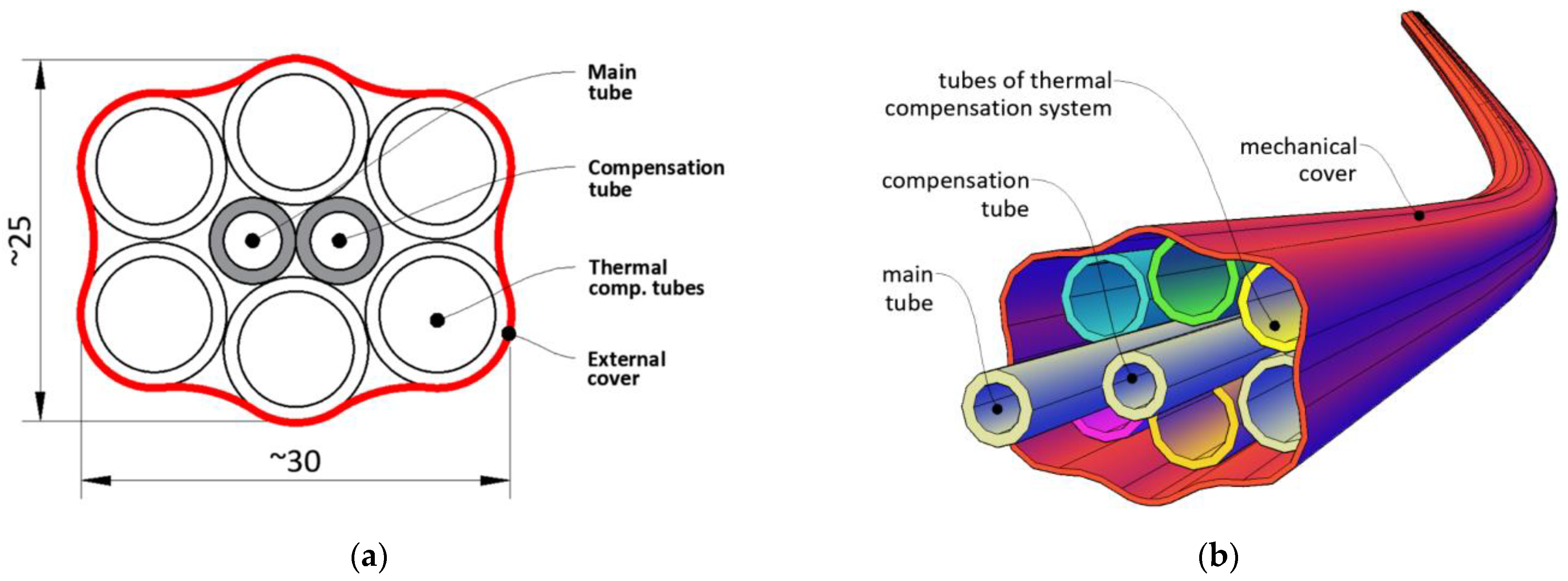
2.3. Sensor Design
- sensor’s performance in difficult geotechnical conditions;
- required accuracy and effectiveness of the thermal compensation system;
- feasibility and ease of establishing a production line;
- low costs of the sensor.
- main tube filled with measuring liquid separated with air bubble. The liquid was pumped with a specified spatial resolution in order to perform the pressure measurements when the height (shape of the sensor) varied along the length;
- compensation tube filled the same way as the main tube; however, the liquid with air bubble was fixed to compensate for all effects affecting pressure measurements, which were not related to change in height (shape) of the sensor. The readings from the compensation tube were subtracted from the main tube in each measuring position;
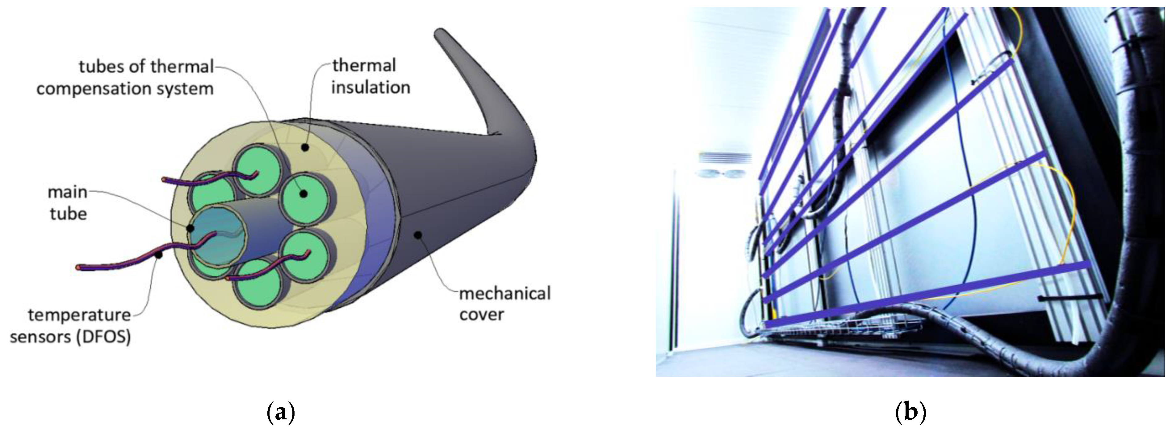
- a set of six tubes filled with the liquid circulating in a closed circuit, the purpose of which was to balance (equalize) the temperature over the entire sensor length. Constant temperature in length domain (not necessarily in time domain) is one of the most important factors providing required accuracy;
- external cover, whose main aim was to protect the sensor’s components against mechanical damages and aggressive and harsh environmental conditions, as well as facilitate the transportation and installation process.
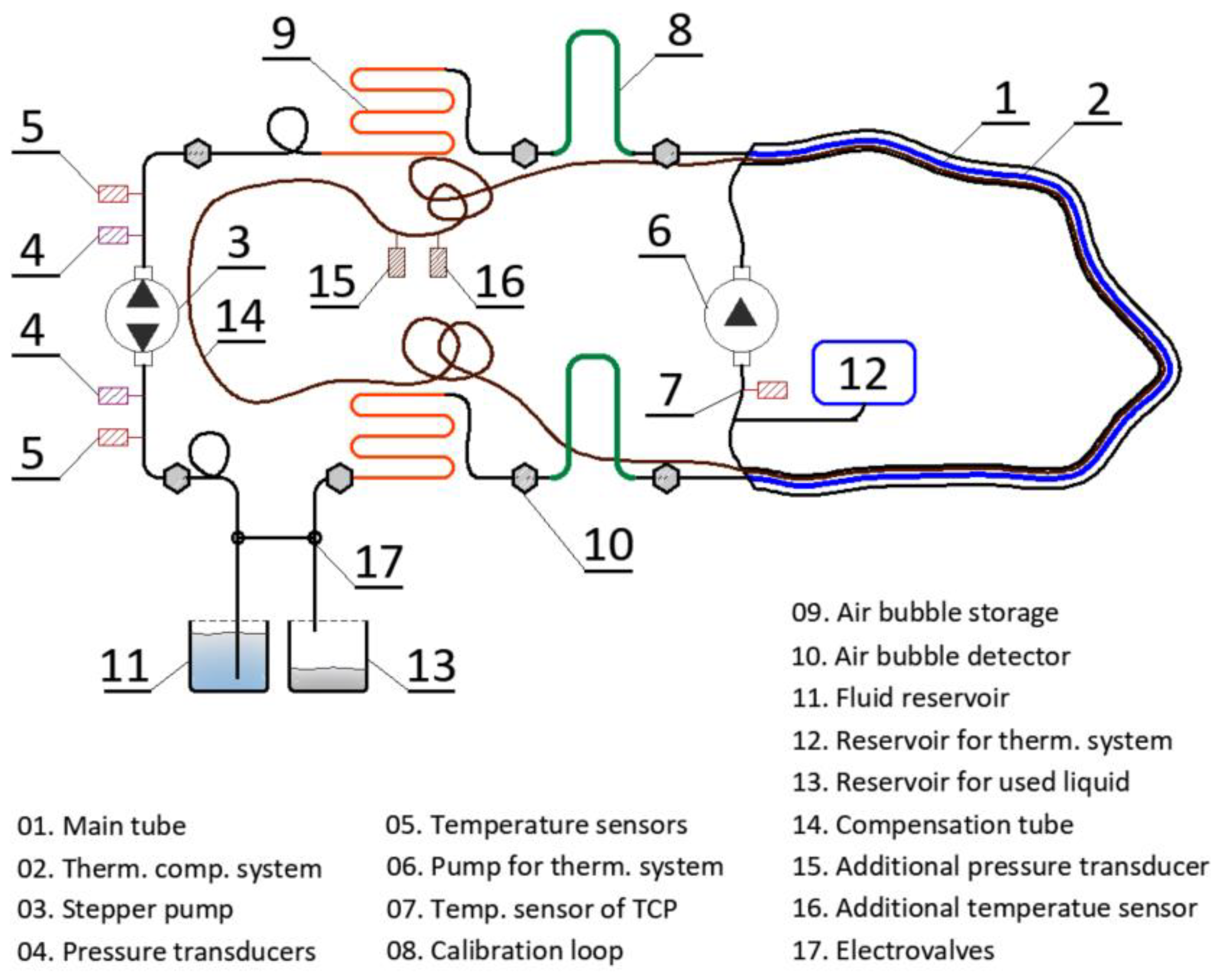
2.4. Hydraulic System (Data-Logger)
3. Laboratory Studies
3.1. Displacements Accuracy
- Based on calibration loops located at the beginning and at the end of the measurement length, whose aim was to eliminate the constant error related to actual conditions during measurement session;
- Compensating for the positioning error resulting from the limited accuracy of applied stepper pump. Based on local approximation approach [22], it was possible to estimate the sought values of displacement at fixed checkpoints, no matter the real measurement positions are. This algorithm is important not only due to the pump precision but also due to possible large displacements significantly changing the geometry of the sensor and, thus, the locations of measuring points within horizontal axis.
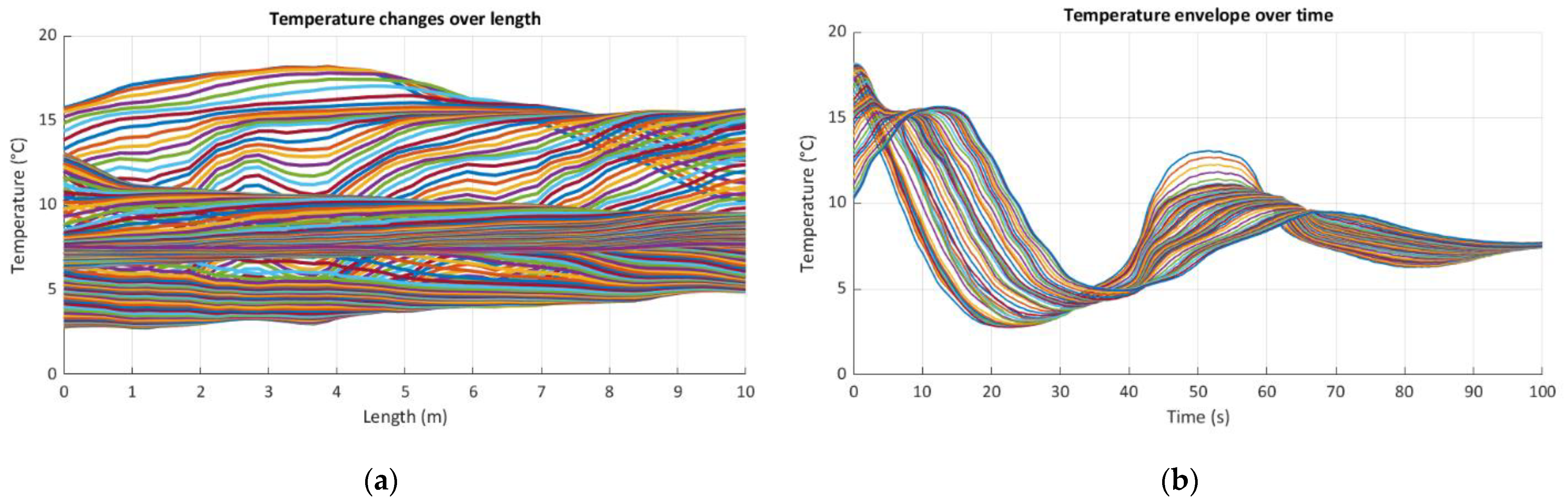
3.2. Thermal Compensation System (TCS)
- a range of spot techniques: fiber Bragg gratings [27], conventional thermistors.
- Continuity equation expressing the principle of mass conservation;
- Equation describing the fluid velocity vector, resulting from Newton’s second law;
- Equation describing the principle of conservation of energy, expressed not directly by the internal energy but by the enthalpy of the volume element.
4. In situ Application
4.1. General Description
4.2. Sensor Delivery, Location, and Installation
4.3. Measurement Sessions
4.4. Example Results and Discussion
5. Conclusions
- Shortening of the duration of construction works by early information about compaction level;
- Possible quality improvement of the works carried out by subcontractors,
- Verification of design assumptions and theoretical simplifications,
- Optimization of technological solutions applied in the future for similar projects,
- Identification of risks and possible reasons for failures,
- Providing objective documentation in case of warranty disputes,
- Improving the positive image and increasing trust in the general contractor.
6. Patents
Author Contributions
Funding
Institutional Review Board Statement
Informed Consent Statement
Data Availability Statement
Conflicts of Interest
References
- Balageas, D.; Fritzen, C.P.; Güemes, A. Structural Health Monitoring; John Wiley & Sons: Hoboken, NJ, USA, 2006; ISBN 978-1-905-20901-9. [Google Scholar]
- Minardo, A.; Persichetti, G.; Testa, G.; Zeni, L.; Bernini, R. Long term structural health monitoring by Brillouin fibre-optic sensing: A real case. J. Geophys. Eng. 2012, 9, S64–S69. [Google Scholar] [CrossRef]
- Faber, M.H. Statistics and Probability Theory in Pursuit of Engineering Decision Support; Springer: Berlin/Heidelberg, Germany, 2012; ISBN 978-94-007-4055-6. [Google Scholar]
- Raiffa, H.; Schlaifer, R. Applied Statistical Decision Theory; John Wiley & Sons: Hoboken, NJ, USA, 2000; ISBN 978-0-471-38349-9. [Google Scholar]
- Xu, Y.L.; Xia, Y. Structural Health Monitoring of Long-Span Suspension Bridges; Spon Press: London, UK, 2012; ISBN 9781138075634. [Google Scholar]
- Kishk, M.; Al-Hajj, A.; Pollock, R.; Bakis, N.; Aouad, G.F.; Bakis, N. Whole-life costing in construction—a state of the art review. RICS Res. Pap. Ser. 2002, 4, 1–52. Available online: https://rgu-repository.worktribe.com/output/248559/whole-life-costing-in-construction-a-state-of-the-art-review (accessed on 2 July 2021).
- Di Sante, R. Fibre Optic Sensors for Structural Health Monitoring of Aircraft Composite Structures: Recent Advances and Applications. Sensors 2015, 15, 18666–18713. [Google Scholar] [CrossRef] [PubMed]
- Guo, H.; Xiao, G.; Mrad, N.; Yao, J. Fiber Optic Sensors for Structural Health Monitoring of Air Platforms. Sensors 2011, 11, 3687–3705. [Google Scholar] [CrossRef] [PubMed]
- Soga, K.; Luo, L. Distributed fiber optics sensors for civil engineering infrastructure sensing. J. Struct. Integr. Maint. 2018, 3, 1–21. [Google Scholar] [CrossRef]
- Hong, C.-Y.; Zhang, Y.-F.; Li, G.-W.; Zhang, M.-X.; Liu, Z.-X. Recent progress of using Brillouin distributed fiber optic sensors for geotechnical health monitoring. Sens. Actuators A Phys. 2017, 258, 131–145. [Google Scholar] [CrossRef]
- DiBiago, E. A Case study of Vibrating-Wire Sensors That Have Vibrated Continuously for 27 Years. In Proceedings of the International symposium on field measurements in geomechanics, Oslo, Norway, 23–26 September 2003. [Google Scholar]
- Cieplok, G.; Bednarski, Ł. Measurements of Dynamic Deformations of Building Structures by Applying Wire Sensors. Sensors 2019, 19, 255. [Google Scholar] [CrossRef] [PubMed] [Green Version]
- Bassil, A.; Wang, X.; Chapeleau, X.; Niederleithinger, E.; Abraham, O.; LeDuc, D. Distributed Fiber Optics Sensing and Coda Wave Interferometry Techniques for Damage Monitoring in Concrete Structures. Sensors 2019, 19, 356. [Google Scholar] [CrossRef] [PubMed] [Green Version]
- Sieńko, R.; Zych, M.; Bednarski, Ł.; Howiacki, T. Strain and crack analysis within concrete members using distributed fibre optic sensors. Struct. Health Monit. 2018, 18, 1510–1526. [Google Scholar] [CrossRef]
- Zhou, D.-P.; Li, W.; Chen, L.; Bao, X. Distributed Temperature and Strain Discrimination with Stimulated Brillouin Scattering and Rayleigh Backscatter in an Optical Fiber. Sensors 2013, 13, 1836–1845. [Google Scholar] [CrossRef] [PubMed] [Green Version]
- Bao, X.; Chen, L. Recent Progress in Brillouin Scattering Based Fiber Sensors. Sensors 2011, 11, 4152–4187. [Google Scholar] [CrossRef] [PubMed]
- Liu, Y.; Li, X.; Li, H.; Fan, X. Global Temperature Sensing for an Operating Power Transformer Based on Raman Scattering. Sensors 2020, 20, 4903. [Google Scholar] [CrossRef] [PubMed]
- Barrias, A.J.D.S.; Casas, J.R.; Villalba, S. A Review of Distributed Optical Fiber Sensors for Civil Engineering Applications. Sensors 2016, 16, 748. [Google Scholar] [CrossRef] [PubMed] [Green Version]
- Lhotzky, K.; Frield, G. Hydrostatic Measuring Method Opens Innovative Possibilities in Geotechnics; Offprint Publication of the DGGT-Special Section-Conference Synthetic Materials in Geotechnics: München, Germany, 2003. [Google Scholar]
- Multipoint Settlement Gauges. Available online: https://www.sisgeo.com/products/settlement-gauges/item/dsm-embankment-settlement-gauge.html (accessed on 18 May 2021).
- Settlement System (VW). Available online: https://www.geokon.com/4660 (accessed on 18 May 2021).
- Bednarski, Ł.; Milewski, S.; Sieńko, R. Determination of vertical and horizontal soil displacements in automated measuring systems on the basis of angular measurements. Tech. Trans. 2014, 6-B, 3–13. [Google Scholar]
- Derkowski, W.; Sieńko, R.; Walczak, R.; Howiacki, T.; Bednarski, Ł. DFOS measurements for strain analysis of anchorage zone in 57-year-old post-tensioned precast concrete girder using static and high-frequency approach. Struct. Concr. 2021, in press. [Google Scholar]
- Sang, A.K.; Froggatt, M.E.; Kreger, S.T.; Gifford, D.K. Millimeter resolution distributed dynamic strain measurements using optical frequency domain reflectometry. In Proceedings of the 21st International Conference on Optical Fiber Sensors, Ottawa, ON, Canada, 15–19 May 2011. [Google Scholar] [CrossRef]
- Funnel, A.; Xu, X.; Yan, J.; Soga, K. Simulation of Noise Within BOTDA and COTDR Systems to Study the Impact on Dynamic Sensing. Int. J. Smart Sens. Intell. Syst. 2015, 8, 1576–1600. [Google Scholar] [CrossRef] [Green Version]
- Wang, W.; Chang, J.; Lv, G.; Wang, Z.; Liu, Z.; Luo, S.; Jiang, S.; Liu, X.; Liu, X.; Liu, Y. Wavelength dispersion analysis on fiber-optic Raman distributed temperature sensor system. Photon. Sens. 2013, 3, 256–261. [Google Scholar] [CrossRef] [Green Version]
- Lin, Y.B.; Chang, K.; Chern, J.C.; Wang, A.L. The health monitoring of a prestressed concrete beam by using fiber Bragg grating sensors. Smart Mater. Struct. 2004, 13, 712–718. [Google Scholar] [CrossRef] [Green Version]
- NERVE Composite DFOS Sensors. Available online: http://nerve-sensors.com (accessed on 25 May 2021).
- Kulpa, M.; Howiacki, T.; Wiater, A.; Siwowski, T.; Sieńko, R. Strain and displacement measurement based on distributed fibre optic sensing (DFOS) system integrated with FRP composite sandwich panel. Measurement 2021, 175, 109099. [Google Scholar] [CrossRef]
- Sieńko, R.; Bednarski, Ł.; Howiacki, T.; Zuiak, K.; Labocha, S. Possibilities of composite distributed fibre optic 3DSensor on the example of footing pulled out from the ground: A case study. In Proceedings of the 8th Civil Structural Health Monitoring Workshop (CSHM-8), Naples, Italy, 29–31 March 2021. [Google Scholar]


| No | Issue | Work Description | Solution/Result |
|---|---|---|---|
| 1 | material of the tube, internal diameter of the tube, type (parameters) of liquid | statistical laboratory research on different materials, diameters, and liquids | selection of the tube’s material, internal diameter, and type of the liquid |
| 2 | long-term operation and aging of the system’s components | aging chamber tests and measurements during specified number of cycles | proved negligible influence of aging in predicted operation time |
| 3 | the minimum length of air bubble not influencing the pressures measured by two transducers on both sides | statistical laboratory research including pressure measurements with different lengths of air bubble at specified heights | empirical equation describing the relation between the max. measurement range and the required length of air bubble |
| 4 | maximum aeration of the liquid allowing for correct measurements | statistical laboratory research on performance of the liquids with different level of aeration measured by dedicated probe | application of air bubble detectors and elaboration of the procedure of automatic exchange of the liquid |
| 5 | the constant temperature along the sensor’s length for correct thermal compensation | verification of the effectiveness of the various systems for temperature equalization within dual-zone thermal chamber—see Section 3.2 | application of special system involving external tubes around the main measuring and compensating tubes—see Section 2.3 |
| 6 | thermal compensation due to the temperature changes between subsequent sessions | analysis of the state-of-the-art, analytical analysis and mathematical models checked under laboratory conditions | set of algorithms for thermal compensation; application of additional compensating tube—see Section 2.3 |
| 7 | numerical model for optimization of the elements dedicated for thermal compensation | simulations using finite element method; nonlinear model based on volume elements and heat transfer equations | possible removal of thermal insulation, support and confirmation of results obtained from laboratory tests |
| 8 | compensation of the positioning error resulting from the limited accuracy of applied stepper pumps and actual geometry of the sensor | theoretical analysis involving mathematical–physical model with local approximation, confirmed by laboratory tests | algorithm for estimation displacements at any reference point, regardless of the actual measurement points |
| 9 | real accuracy of displacement profile measurements | statistical laboratory research under the control of reference, independent techniques for displacement measurements—see Section 3.1 | data sheet and technical specifications of the new sensor |
| 10 | connection of the sensor’s segments to avoid destruction of air bubble | statistical laboratory research on different types of hydraulic connectors and methods of cutting off the tube face | elaboration of the optimum way to connect the sensor |
| 11 | data acquisition system | collaboration of interdisciplinary specialists to create electronic-information–hydraulic system | devices and software allowed to perform measurements remotely, automatically and without operator |
| 12 | verification of sensor performance in harsh environmental conditions | sensors’ demonstration installations in field conditions (one bridge and two geotechnical structures—embankments) | installation, measurements, data processing, real performance → lessons learned (see also Section 4) |
| Session | Data Uncorrected | Data Corrected | ||||
|---|---|---|---|---|---|---|
| h(12) | h(13) | h(23) | h(12) | h(13) | h(23) | |
| S00 | 0.4 | 1.1 | 1.6 | 0.1 | 0.0 | 0.1 |
| S01 | 0.4 | 0.9 | 1.4 | 0.2 | 0.2 | 0.3 |
| S02 | 0.3 | 1.1 | 1.7 | 0.0 | 0.1 | 0.1 |
| S03 | 0.4 | 1.1 | 1.6 | 0.1 | 0.0 | 0.0 |
| S04 | 0.5 | 1.1 | 1.5 | 0.1 | 0.1 | 0.1 |
| S05 | 0.5 | 1.1 | 1.5 | 0.2 | 0.3 | 0.1 |
| Mean | 0.4 | 1.1 | 1.6 | 0.1 | 0.1 | 0.1 |
| Stdv 3 | 0.1 | 0.1 | 0.1 | 0.1 | 0.1 | 0.1 |
| Parameter | Value |
|---|---|
| Range of displacement measurement | up to 9 m |
| Accuracy of displacement measurement | <1.0% f.s. |
| Resolution of displacement measurement | ±1 mm |
| Spatial resolution 1 | >5 cm |
| Operation temperature 2 | from −20 °C to +60 °C |
| Cross section dimensions | 25 × 30 mm |
| Measurement length | up to 300 m |
| Weight of the sensor | 0.5 kg/m |
Publisher’s Note: MDPI stays neutral with regard to jurisdictional claims in published maps and institutional affiliations. |
© 2021 by the authors. Licensee MDPI, Basel, Switzerland. This article is an open access article distributed under the terms and conditions of the Creative Commons Attribution (CC BY) license (https://creativecommons.org/licenses/by/4.0/).
Share and Cite
Bednarski, Ł.; Sieńko, R.; Kanty, P.; Howiacki, T. New Hydraulic Sensor for Distributed and Automated Displacement Measurements with Temperature Compensation System. Sensors 2021, 21, 4678. https://doi.org/10.3390/s21144678
Bednarski Ł, Sieńko R, Kanty P, Howiacki T. New Hydraulic Sensor for Distributed and Automated Displacement Measurements with Temperature Compensation System. Sensors. 2021; 21(14):4678. https://doi.org/10.3390/s21144678
Chicago/Turabian StyleBednarski, Łukasz, Rafał Sieńko, Piotr Kanty, and Tomasz Howiacki. 2021. "New Hydraulic Sensor for Distributed and Automated Displacement Measurements with Temperature Compensation System" Sensors 21, no. 14: 4678. https://doi.org/10.3390/s21144678
APA StyleBednarski, Ł., Sieńko, R., Kanty, P., & Howiacki, T. (2021). New Hydraulic Sensor for Distributed and Automated Displacement Measurements with Temperature Compensation System. Sensors, 21(14), 4678. https://doi.org/10.3390/s21144678