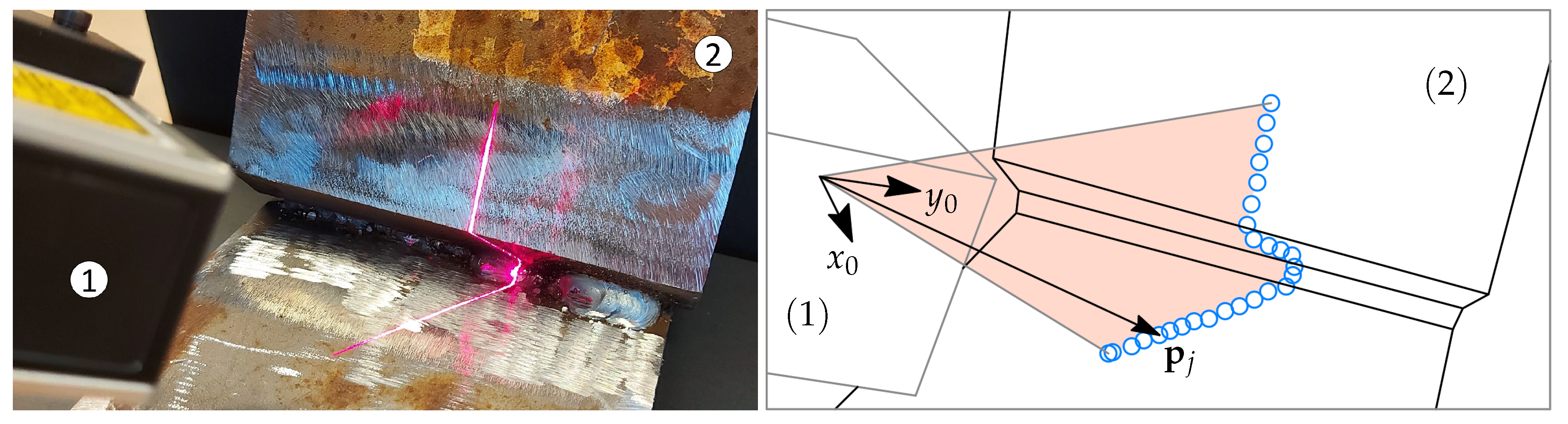
Figure 1.
A commercial laser triangulation sensor (1) pointing at the weld groove of a test object (2). A local sensor fixed frame is denoted Frame 0 and all data points are obtained in the coordinates of Frame 0.
Figure 1.
A commercial laser triangulation sensor (1) pointing at the weld groove of a test object (2). A local sensor fixed frame is denoted Frame 0 and all data points are obtained in the coordinates of Frame 0.
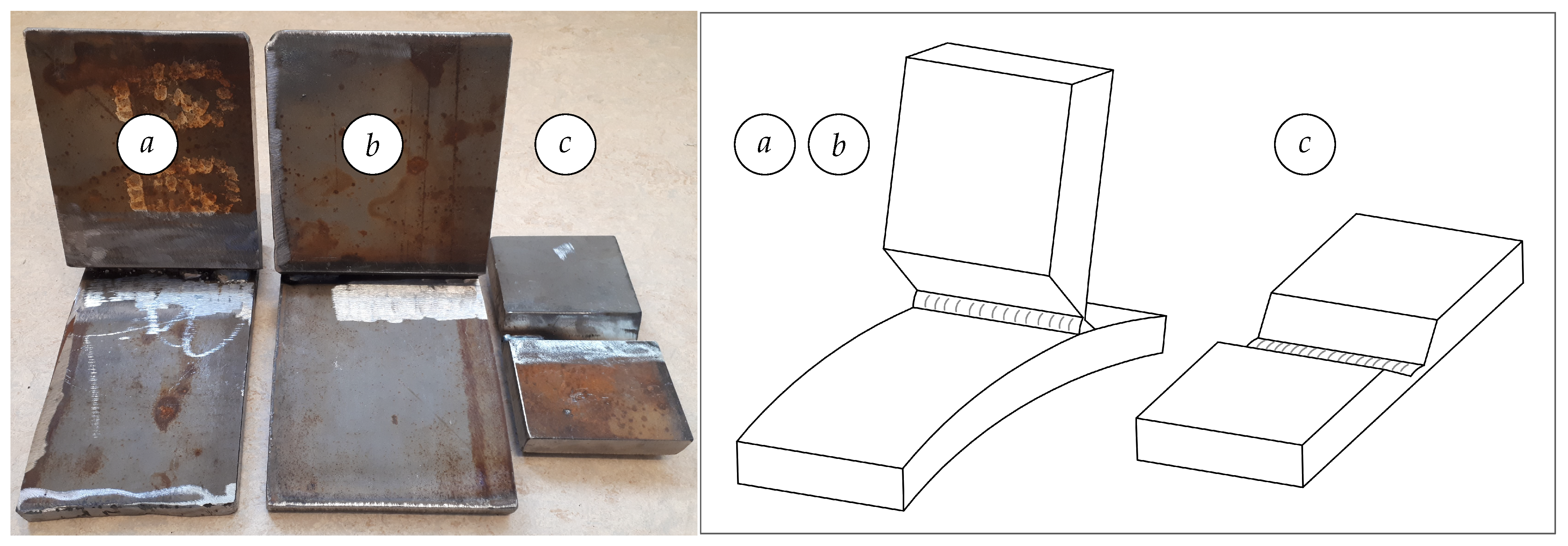
Figure 2.
Three test objects used in the tests. The objects (a) and (b) represent a typical stub–joint groove, while the object (c) represents a typical butt-joint groove. The objects are welded with root welds of different widths. Schematic arrangement of the plates and the weld root pass in the test objects is shown to the right.
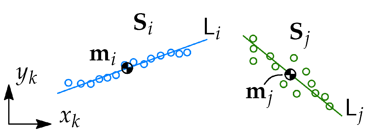
Figure 3.
Two examples of point sets and . Each of the point sets has the center of mass or and the line fit or . The point sets are marked with different color and the line fit is shown using the same colors.
Figure 3.
Two examples of point sets and . Each of the point sets has the center of mass or and the line fit or . The point sets are marked with different color and the line fit is shown using the same colors.
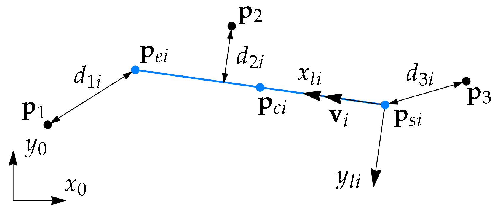
Figure 4.
A line segment i is shown in blue color, with three different cases of point-to-segment distances for .
Figure 4.
A line segment i is shown in blue color, with three different cases of point-to-segment distances for .
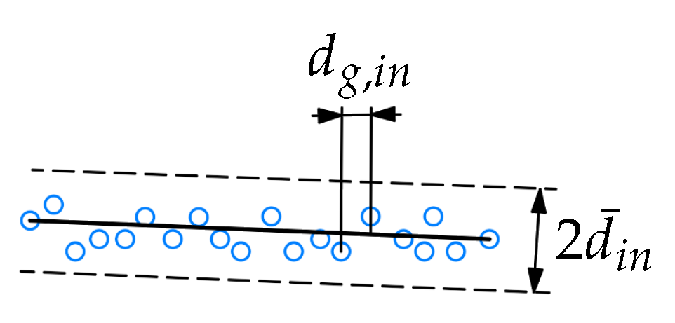
Figure 5.
Inliers for a line segment with the inlier tolerance . The gap between points along the axis is denoted .
Figure 5.
Inliers for a line segment with the inlier tolerance . The gap between points along the axis is denoted .
Figure 6.
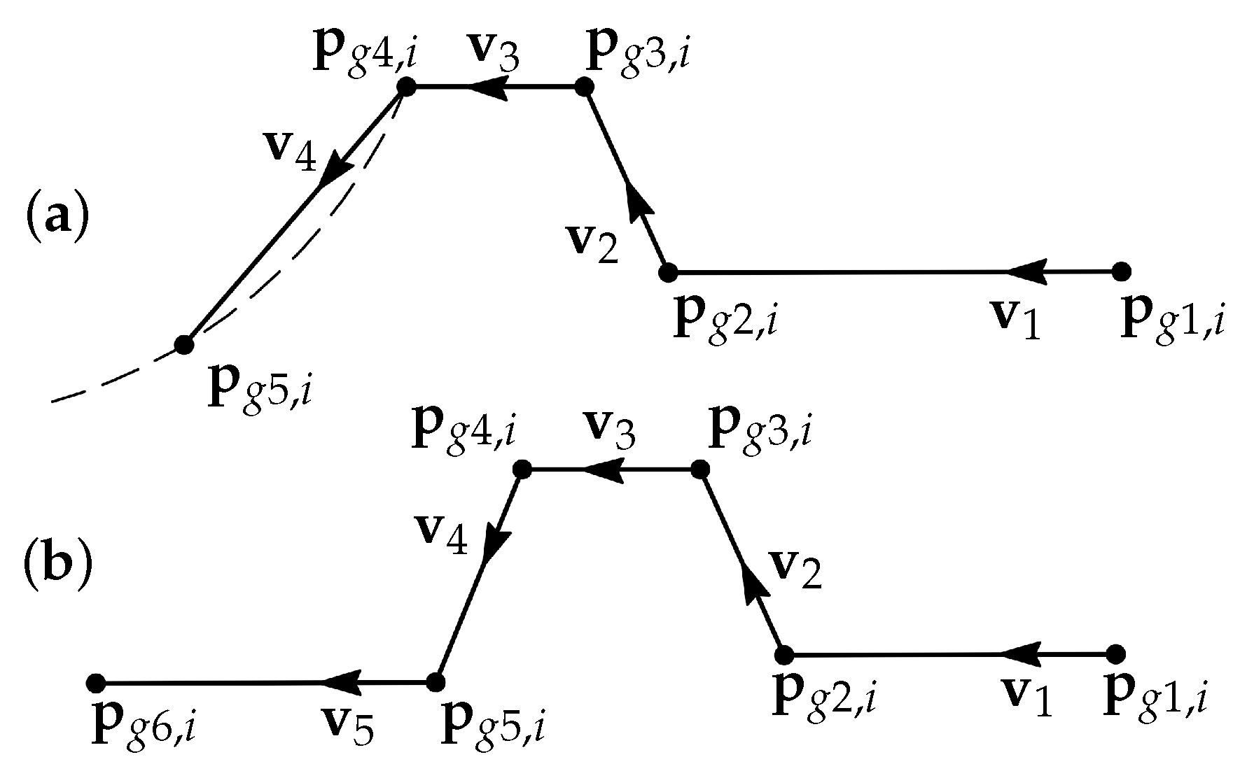
Two models for groove profiles: (a) a T-joint (i.e., stub joint) groove and (b) a butt joint groove (a V-groove) with a root weld. A stub groove and a butt groove consist of five or six corner points, respectively, which can also be represented as four or five sequentially connected line segments. The vectors show the directions of the segments.
Figure 6.
Two models for groove profiles: (a) a T-joint (i.e., stub joint) groove and (b) a butt joint groove (a V-groove) with a root weld. A stub groove and a butt groove consist of five or six corner points, respectively, which can also be represented as four or five sequentially connected line segments. The vectors show the directions of the segments.
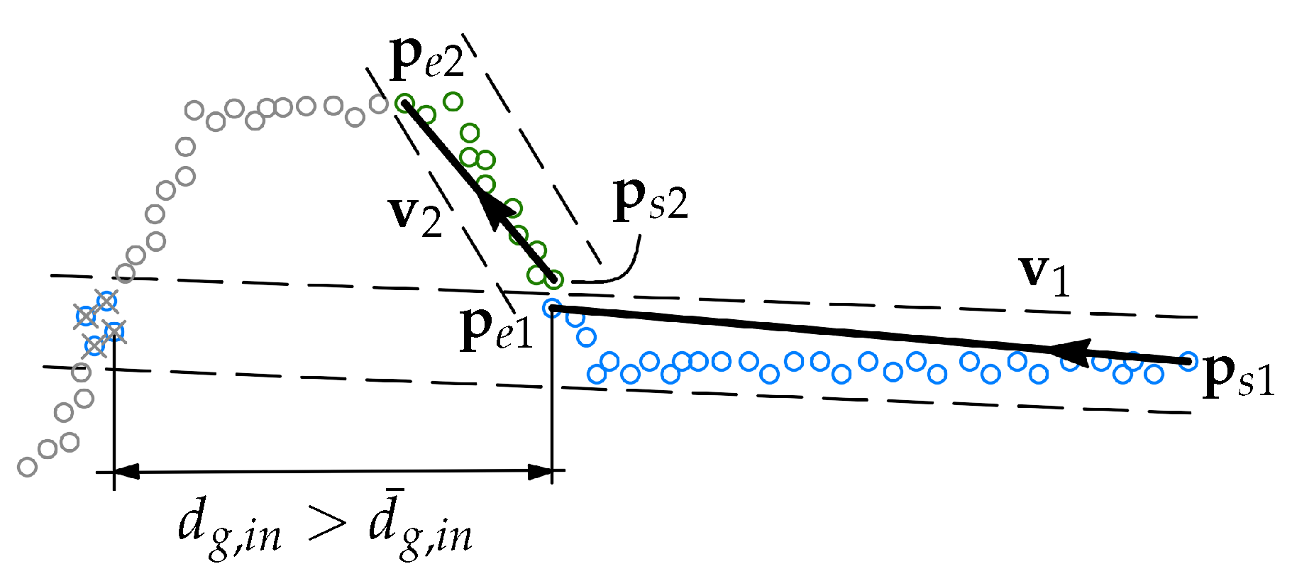
Figure 7.
Procedure of searching the two first line segments using RANSAC. Inliers of segment 1 are shown in blue. These inliers, excluding the inliers separated by the gap , are used for defining the segment. After segment 1 is defined, the best inlier set for segment 2 is found, which is shown in green, and segment 2 is defined.
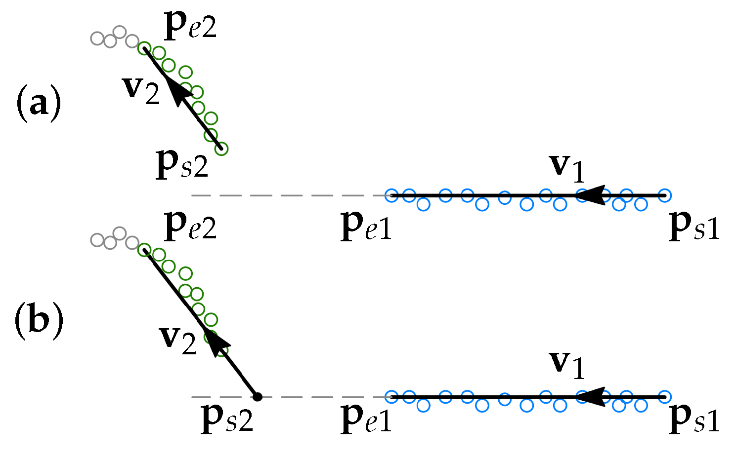
Figure 8.
(a) Two segments 1 and 2 are found. The segments are divided since the gap . (b) If the angle between and is less than the defined angle tolerance , then the two segments are merged.
Figure 8.
(a) Two segments 1 and 2 are found. The segments are divided since the gap . (b) If the angle between and is less than the defined angle tolerance , then the two segments are merged.
Figure 9.
(a) Two segments 1 and 2 are found. (b) If the angle , then the start point is moved to the intersection between the segments 1 and 2.
Figure 9.
(a) Two segments 1 and 2 are found. (b) If the angle , then the start point is moved to the intersection between the segments 1 and 2.
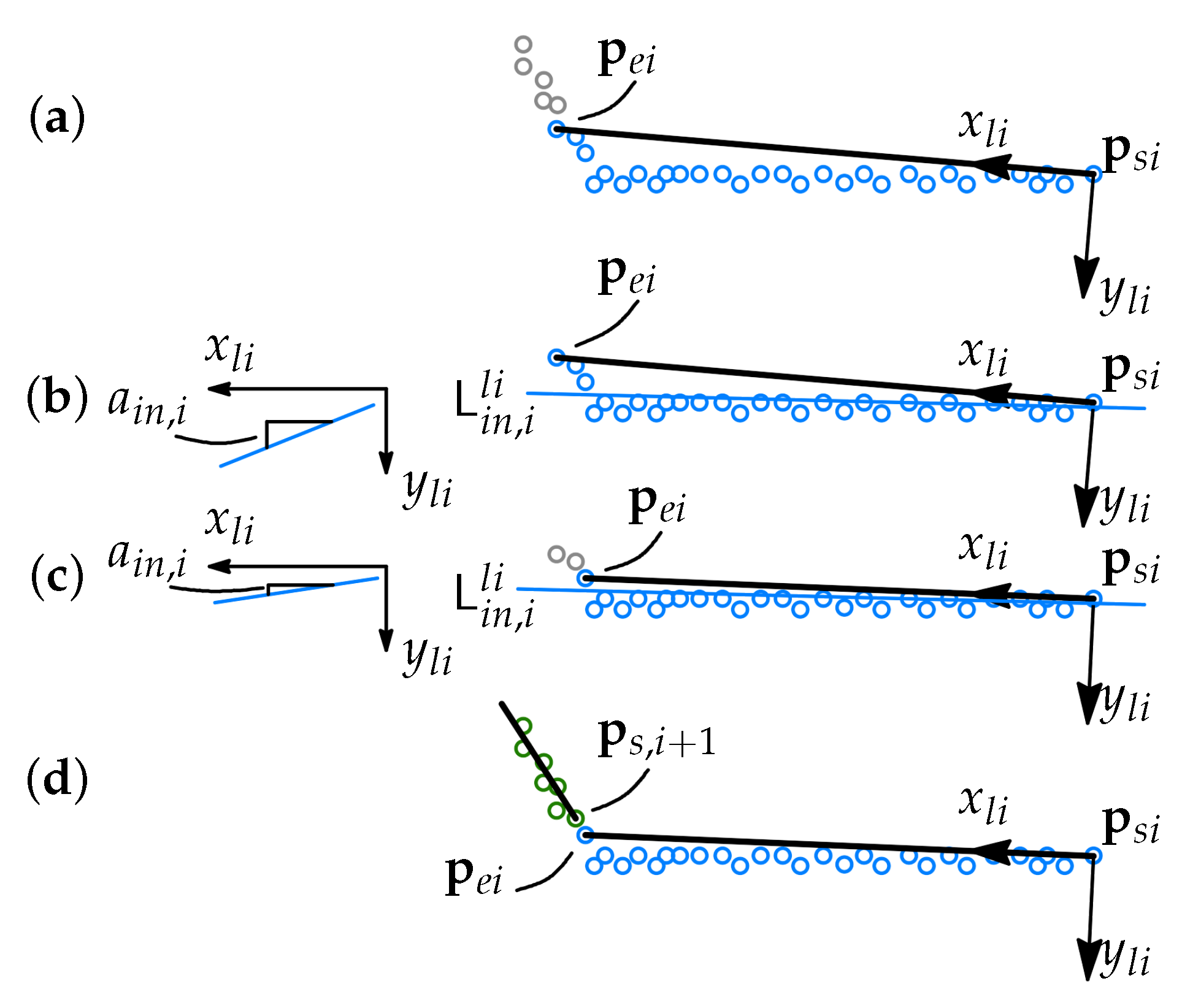
Figure 10.
(a) Segment i and its local Frame are defined over the inlier set, (b) A line fit for the inliers is found and the coefficient of the line equation is evaluated, (c) several points are removed from the inlier set and a line fit is evaluated again, (d) when is within the tolerance, segment i is defined over the rest of the inliers.
Figure 11.
Input data (a) and the output (b) of the iterative error elimination algorithm. The different point colors indicate point sets associated with different segments, initial point association is shown in (a) and after the final iteration—in (b).
Figure 11.
Input data (a) and the output (b) of the iterative error elimination algorithm. The different point colors indicate point sets associated with different segments, initial point association is shown in (a) and after the final iteration—in (b).
Figure 12.
Alignment of segment i to the point set . First the segment is translated to the mass center of , then it is rotated to match the direction of .
Figure 12.
Alignment of segment i to the point set . First the segment is translated to the mass center of , then it is rotated to match the direction of .
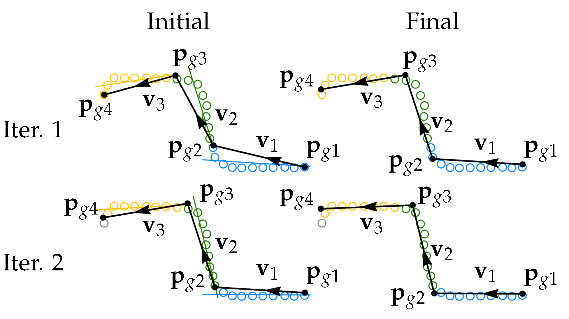
Figure 13.
Schematic representation of the iterative corner error elimination algorithm. Two iterations are shown with the initial and final groove profile arrangements.
Figure 13.
Schematic representation of the iterative corner error elimination algorithm. Two iterations are shown with the initial and final groove profile arrangements.
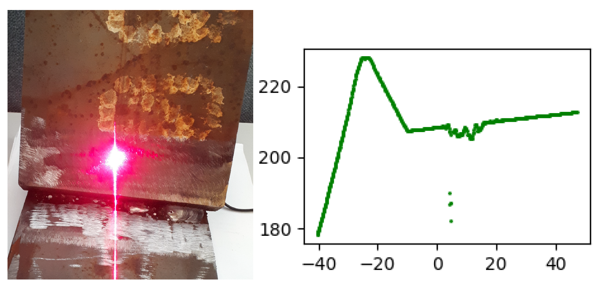
Figure 14.
Reflections from laser projection onto shiny metal surface and the corresponding data noise in the graph.
Figure 14.
Reflections from laser projection onto shiny metal surface and the corresponding data noise in the graph.
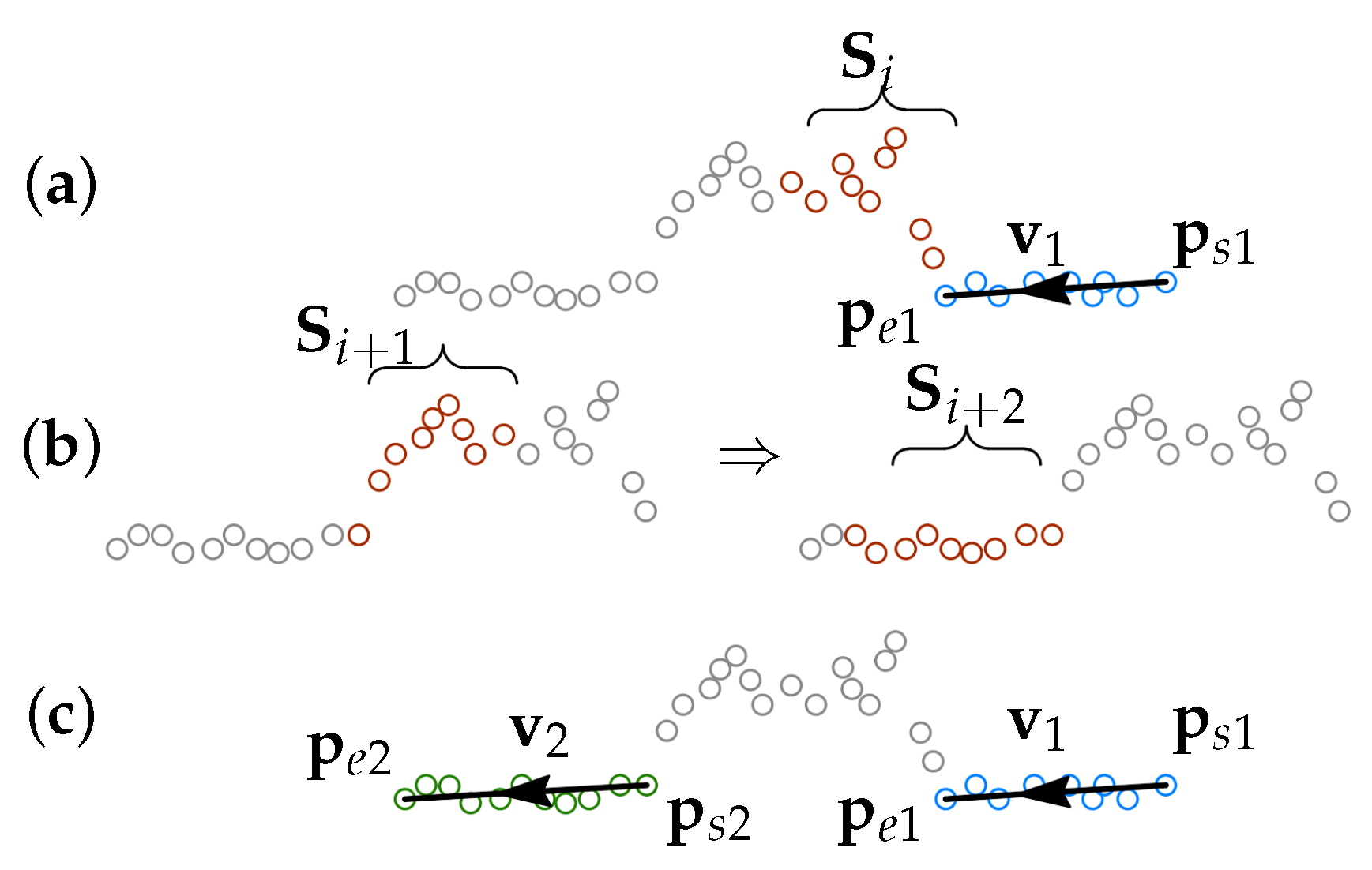
Figure 15.
Schematic representation of the noise detection procedure. When segment 1 is found, the algorithm detects noise in the set of the following points (a), then the following point sets and are checked for noise (b), segment 2 is defined once a noise free set is found (c).
Figure 15.
Schematic representation of the noise detection procedure. When segment 1 is found, the algorithm detects noise in the set of the following points (a), then the following point sets and are checked for noise (b), segment 2 is defined once a noise free set is found (c).
Figure 16.
Flow diagram the proposed procedure for groove parametrization with noisy data points. The diagram does not include the iterative error elimination step.
Figure 16.
Flow diagram the proposed procedure for groove parametrization with noisy data points. The diagram does not include the iterative error elimination step.
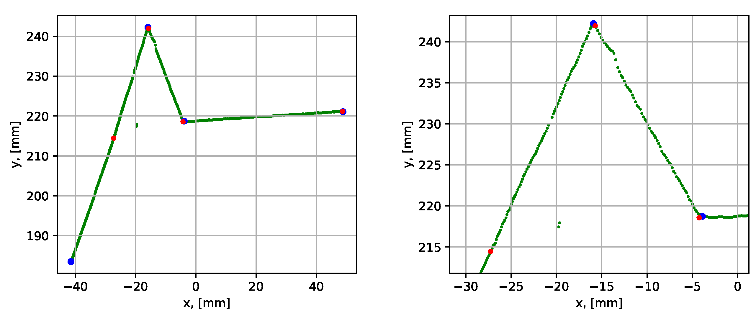
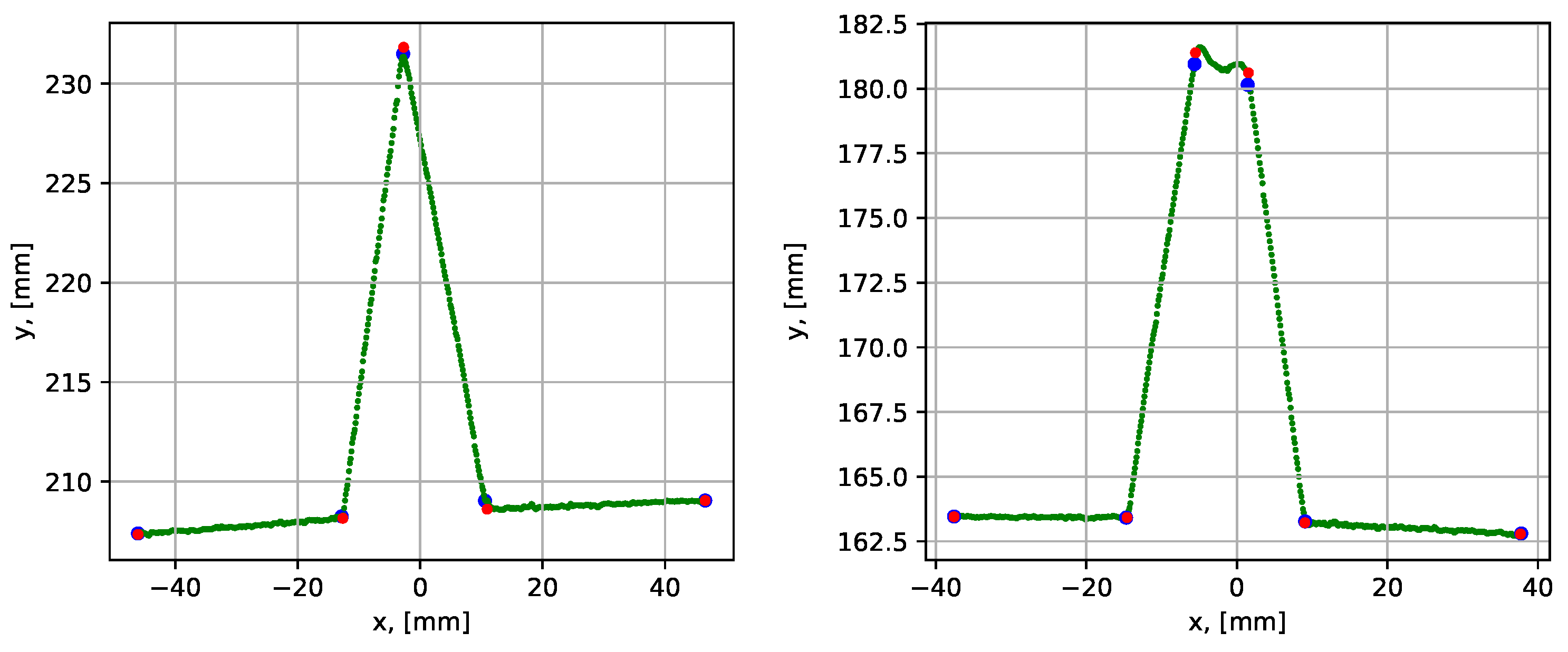
Figure 17.
Parametrization results with groove corner points for dataset 1. The blue dots show the result before the iterative error elimination procedure and the red dots show after. A close-up of the graph is shown to the right.
Figure 17.
Parametrization results with groove corner points for dataset 1. The blue dots show the result before the iterative error elimination procedure and the red dots show after. A close-up of the graph is shown to the right.
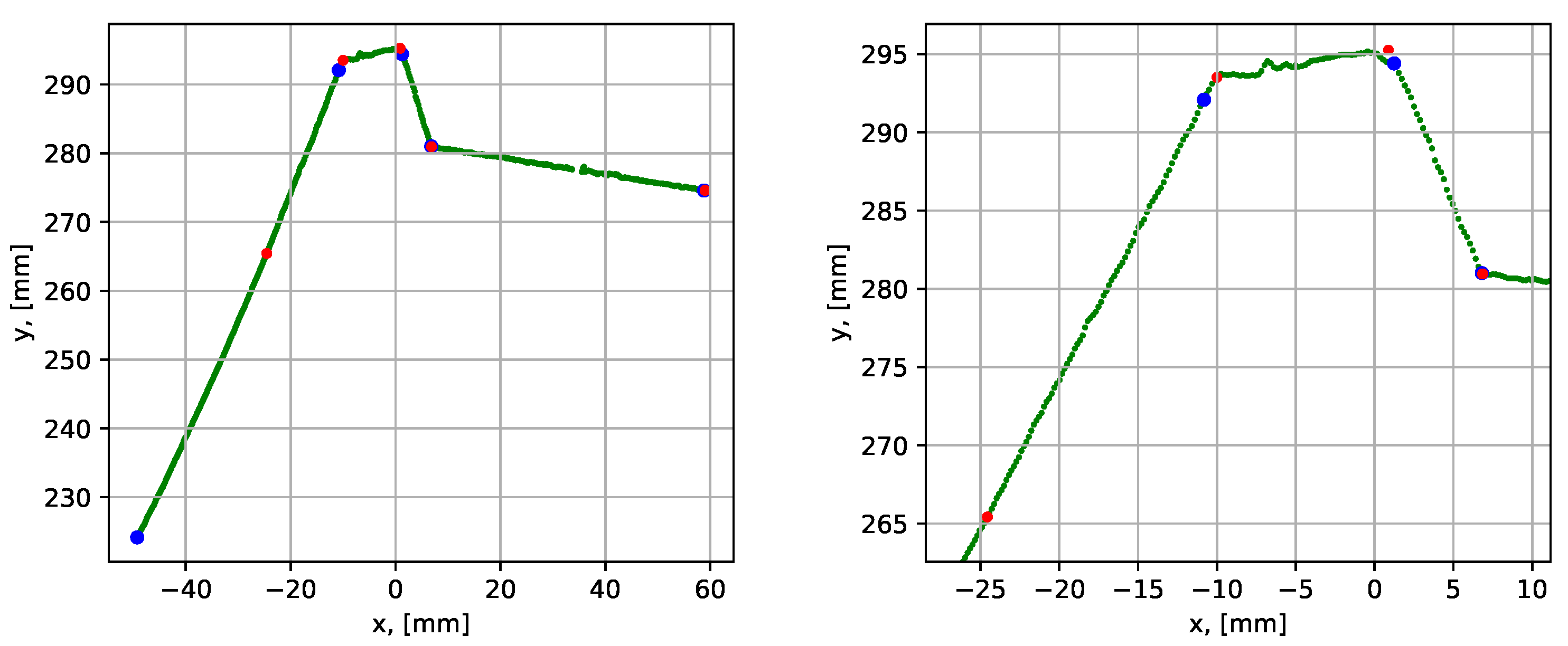
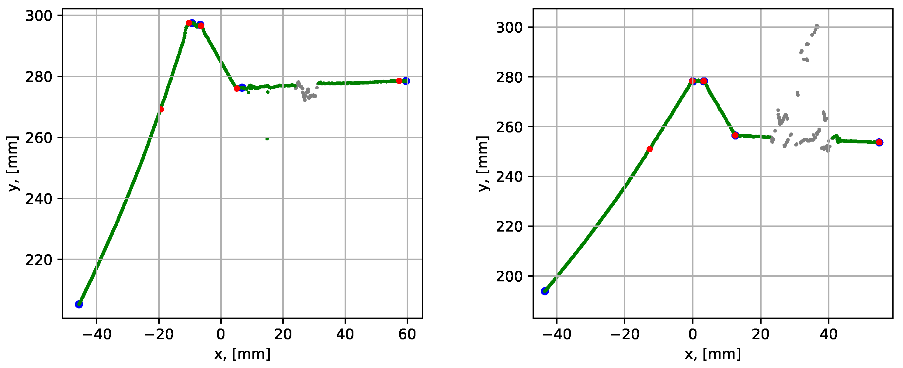
Figure 18.
Parametrization results with groove corner points for dataset 2. The blue dots show the result before the iterative error elimination procedure and the red dots show after. A close-up of the graph is shown to the right.
Figure 18.
Parametrization results with groove corner points for dataset 2. The blue dots show the result before the iterative error elimination procedure and the red dots show after. A close-up of the graph is shown to the right.
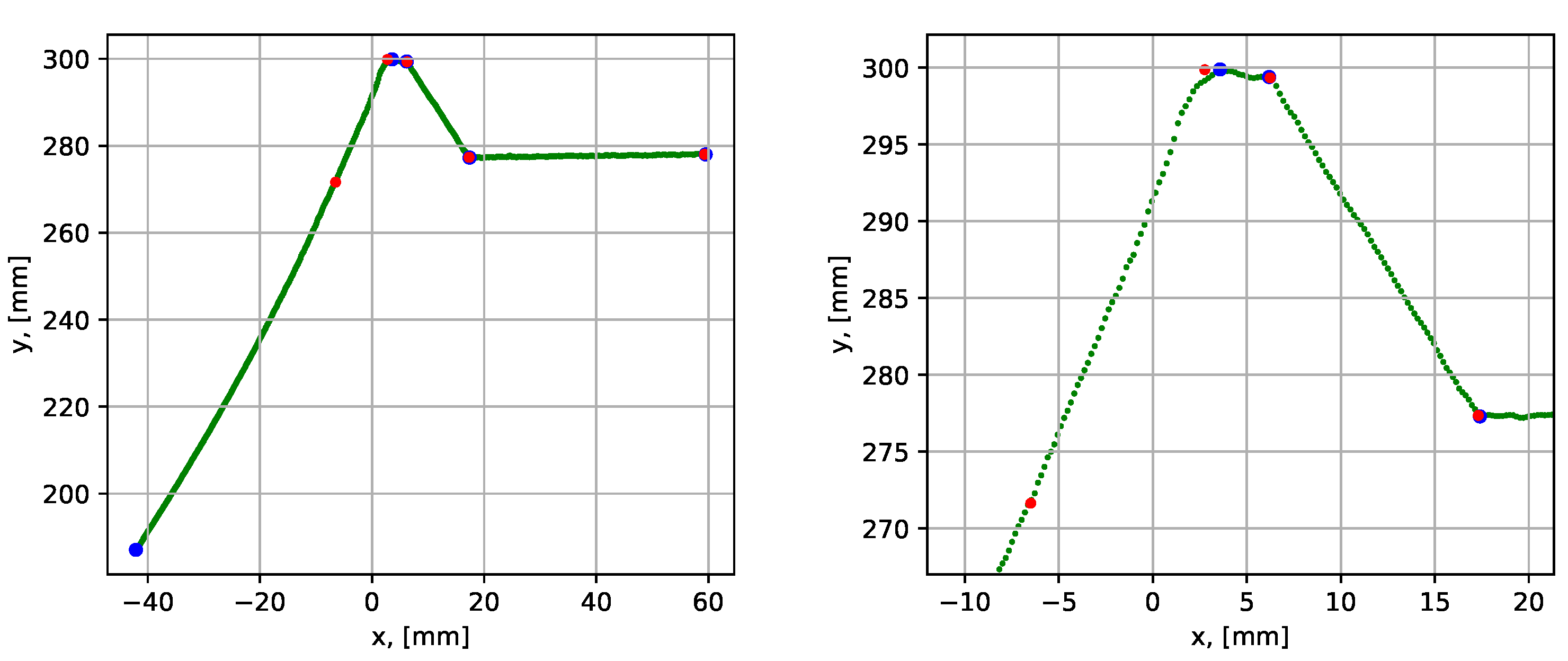
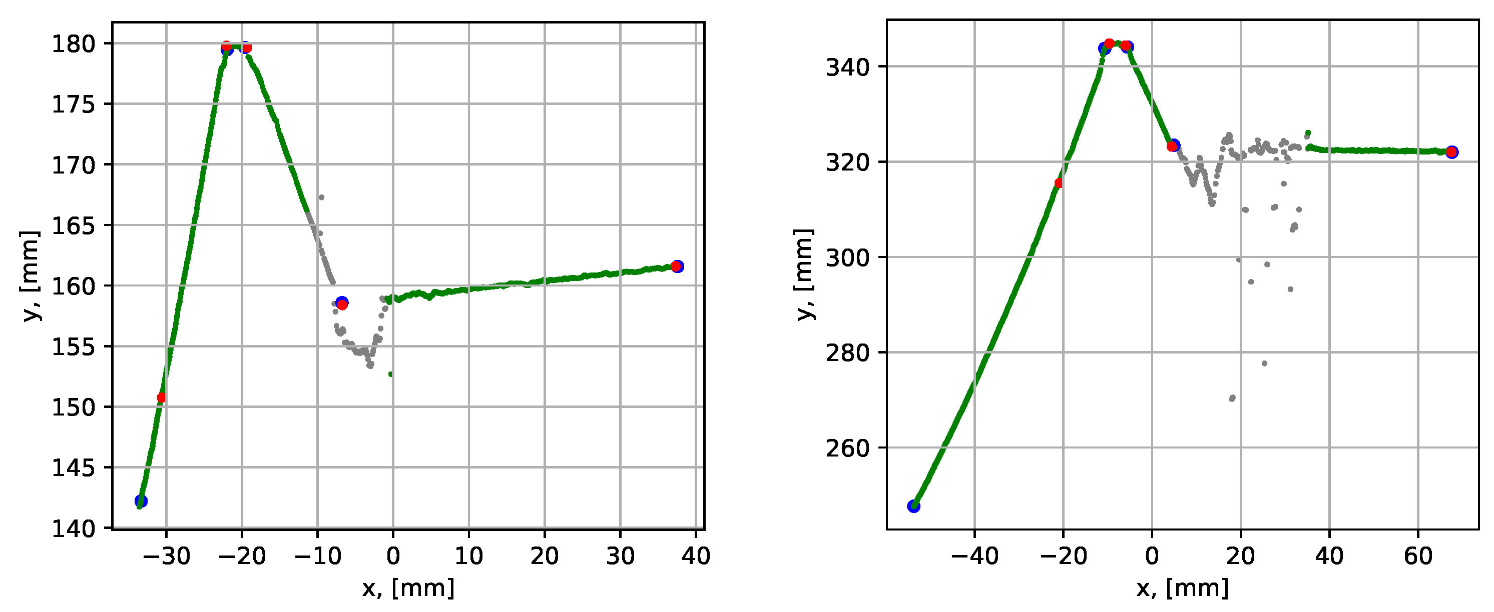
Figure 19.
Parametrization results with groove corner points for dataset 3. The blue dots show the result before the iterative error elimination procedure and the red dots show after. A close-up of the graph is shown to the right.
Figure 19.
Parametrization results with groove corner points for dataset 3. The blue dots show the result before the iterative error elimination procedure and the red dots show after. A close-up of the graph is shown to the right.
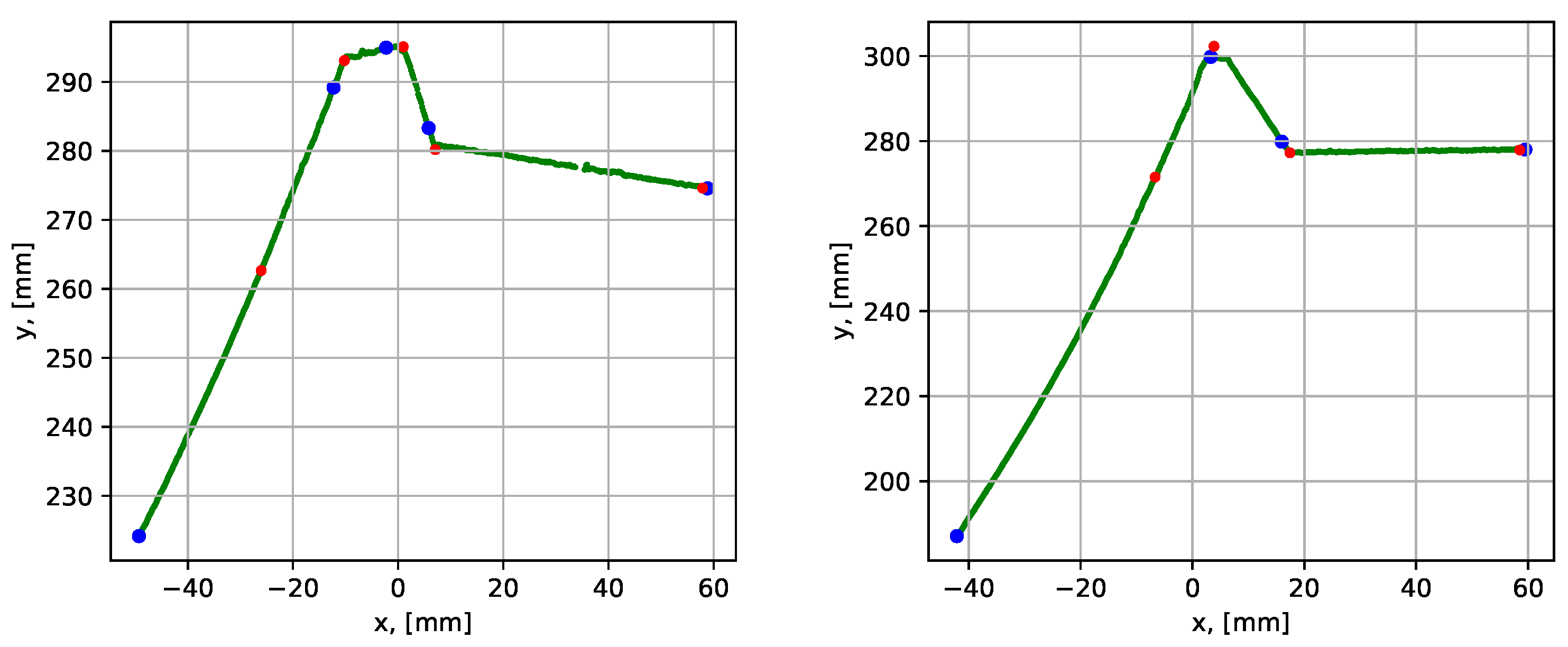
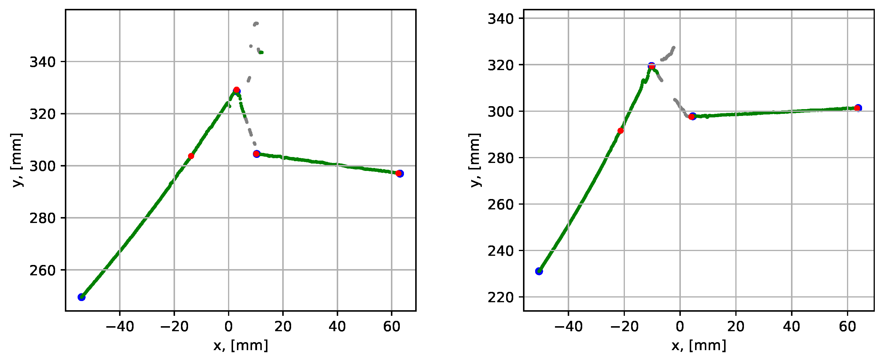
Figure 20.
Parametrization results with groove corner points for dataset 2 (to the left) and 3 (to the right), when the correction of assigned corners step is omitted. The blue dots show the result before the iterative error elimination procedure and the red dots show after.
Figure 20.
Parametrization results with groove corner points for dataset 2 (to the left) and 3 (to the right), when the correction of assigned corners step is omitted. The blue dots show the result before the iterative error elimination procedure and the red dots show after.
Figure 21.
Parametrization results with groove corner points for datasets 4 (to the left) and 5 (to the right). The blue dots show the result before the iterative error elimination procedure and the red dots show after.
Figure 21.
Parametrization results with groove corner points for datasets 4 (to the left) and 5 (to the right). The blue dots show the result before the iterative error elimination procedure and the red dots show after.
Figure 22.
Parametrization results with groove corner points for datasets 6 (to the left) and 7 (to the right). The blue dots show the result before the iterative error elimination procedure and the red dots show after. The grey points have been identified as noise by the noise detection algorithm.
Figure 22.
Parametrization results with groove corner points for datasets 6 (to the left) and 7 (to the right). The blue dots show the result before the iterative error elimination procedure and the red dots show after. The grey points have been identified as noise by the noise detection algorithm.
Figure 23.
Parametrization results with groove corner points for datasets 8 (to the left) and 9 (to the right). The blue dots show the result before the iterative error elimination procedure and the red dots show after. The grey points have been identified as noise by the noise detection algorithm.
Figure 23.
Parametrization results with groove corner points for datasets 8 (to the left) and 9 (to the right). The blue dots show the result before the iterative error elimination procedure and the red dots show after. The grey points have been identified as noise by the noise detection algorithm.
Figure 24.
Parametrization results with groove corner points for datasets 10 (to the left) and 11 (to the right). The blue dots show the result before the iterative error elimination procedure and the red dots show after. The grey points have been identified as noise by the noise detection algorithm.
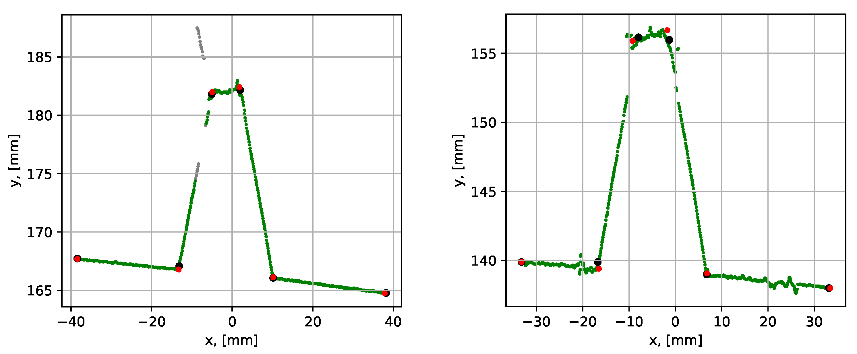
Figure 25.
Parametrization results with groove corner points for datasets 12 (to the left) and 13 (to the right). The red dots show the result from the proposed procedure and the black dots show results from the conventional RANSAC. The grey points have been identified as noise by the noise detection algorithm.
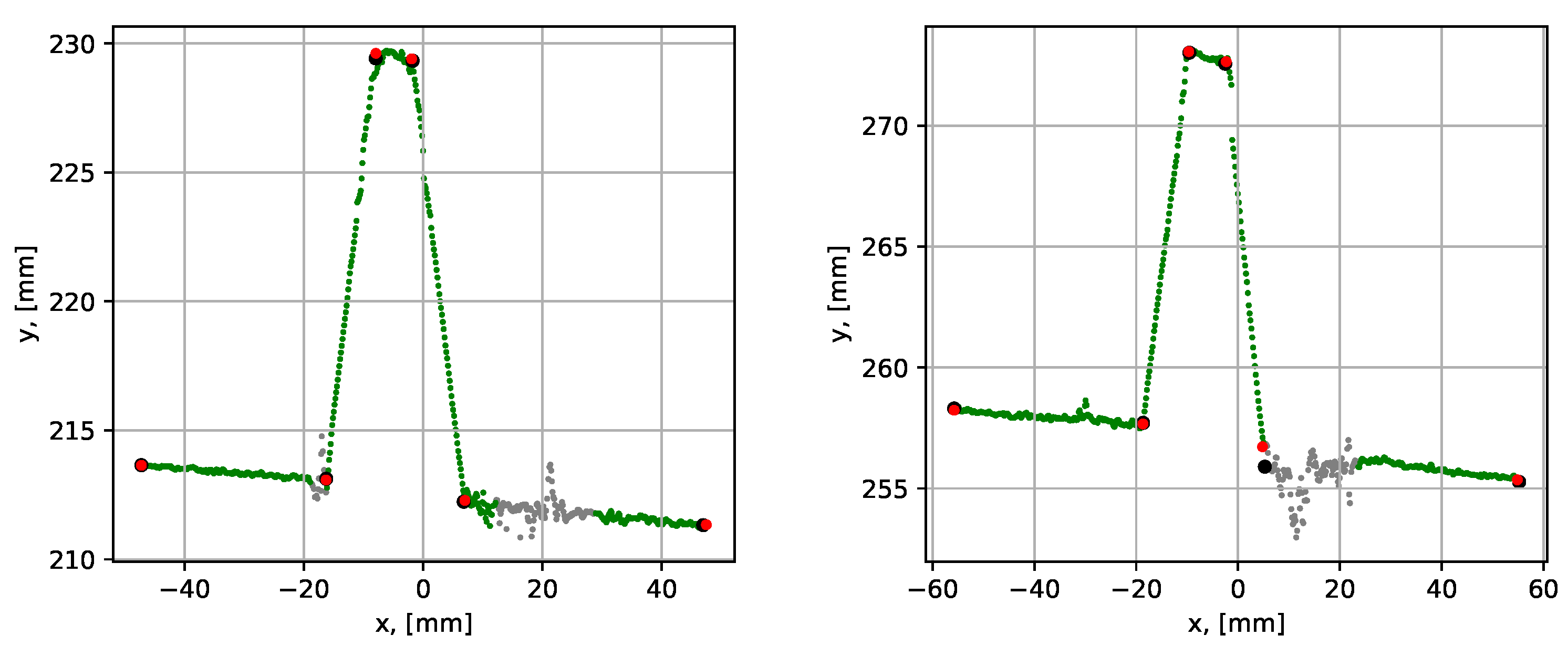
Figure 26.
Parametrization results with groove corner points for datasets 14 (to the left) and 15 (to the right). The red dots show the result from the proposed procedure and the black dots show results from the conventional RANSAC. The grey points have been identified as noise by the noise detection algorithm.
Table 1.
Datasets from the scanned weld grooves.
Table 1.
Datasets from the scanned weld grooves.
| No. | Type | Root, | Noise | No. | Type | Root, | Noise | No. | Type | Root, | Noise |
|---|
| | | [mm] | | | | [mm] | | | | [mm] | |
|---|
| 1 | Stub | 0 | No | 6 | Stub | 3 | Low N1 | 11 | Stub | 0 | Medium N3 |
| 2 | Stub | 11 | No | 7 | Stub | 3 | High N1 | 12 | Butt | 7 | Medium N1 |
| 3 | Stub | 3 | No | 8 | Stub | 3 | Medium N2 | 13 | Butt | 7 | Medium N2 |
| 4 | Butt | 0 | No | 9 | Stub | 3 | High N2 | 14 | Butt | 7 | Medium N3 |
| 5 | Butt | 7 | No | 10 | Stub | 0 | Low N3 | 15 | Butt | 7 | Low N3 |
Table 2.
Segment fit errors and execution times for 10 sequential runs using the datasets 1, 2, and 3. Results for dataset 2 are given with and without iterative error elimination step (IEES). The fit error definition is given in the beginning of
Section 4.
Table 2.
Segment fit errors and execution times for 10 sequential runs using the datasets 1, 2, and 3. Results for dataset 2 are given with and without iterative error elimination step (IEES). The fit error definition is given in the beginning of
Section 4.
| Dataset | 1 | 2 with IEES | 2 without IEES | 3 |
|---|
| | Max | Min | Mean | Max | Min | Mean | Max | Min | Mean | Max | Min | Mean |
|---|
| Time, [s] | 0.076 | 0.043 | 0.061 | 0.125 | 0.056 | 0.092 | - | - | - | 0.145 | 0.058 | 0.126 |
| , [mm] | 0.034 | 0.034 | 0.034 | 0.064 | 0.061 | 0.062 | 0.062 | 0.062 | 0.062 | 0.056 | 0.056 | 0.056 |
| , [mm] | 0.070 | 0.070 | 0.070 | 0.114 | 0.095 | 0.109 | 1.058 | 0.040 | 0.192 | 0.041 | 0.041 | 0.041 |
| , [mm] | 0.050 | 0.050 | 0.050 | 0.123 | 0.115 | 0.118 | 1.152 | 0.122 | 0.740 | 0.095 | 0.095 | 0.095 |
| , [mm] | - | - | - | 0.046 | 0.044 | 0.044 | 0.659 | 0.400 | 0.618 | 0.074 | 0.074 | 0.074 |
Table 3.
Segment fit errors and execution times for 10 sequential runs using datasets 4 and 5. The fit error definition is given in the beginning of
Section 4.
Table 3.
Segment fit errors and execution times for 10 sequential runs using datasets 4 and 5. The fit error definition is given in the beginning of
Section 4.
| Dataset | | 4 | | | 5 | |
|---|
| | Max | Min | Mean | Max | Min | Mean |
|---|
| Time, [s] | 0.138 | 0.062 | 0.091 | 0.233 | 0.093 | 0.142 |
| , [mm] | 0.030 | 0.028 | 0.030 | 0.062 | 0.030 | 0.046 |
| , [mm] | 0.074 | 0.074 | 0.074 | 0.077 | 0.026 | 0.052 |
| , [mm] | 0.036 | 0.035 | 0.036 | 0.161 | 0.160 | 0.160 |
| , [mm] | 0.032 | 0.032 | 0.032 | 0.042 | 0.041 | 0.041 |
| , [mm] | - | - | - | 0.019 | 0.019 | 0.019 |
Table 4.
Segment fit errors and running times for 10 sequential runs using the datasets 6–11. The fit error definition is given in the beginning of
Section 4.
Table 4.
Segment fit errors and running times for 10 sequential runs using the datasets 6–11. The fit error definition is given in the beginning of
Section 4.
| Dataset | 6 | 7 | 8 | 9 | 10 | 11 |
|---|
| | Max | Mean | Max | Mean | Max | Mean | Max | Mean | Max | Mean | Max | Mean |
|---|
| Time, [s] | 0.133 | 0.126 | 0.262 | 0.139 | 0.089 | 0.061 | 0.133 | 0.108 | 0.162 | 0.125 | 0.066 | 0.046 |
| , [mm] | 0.258 | 0.258 | 0.178 | 0.115 | 0.086 | 0.086 | 0.106 | 0.105 | 0.077 | 0.077 | 0.070 | 0.070 |
| , [mm] | 0.144 | 0.141 | 0.040 | 0.040 | 0.078 | 0.076 | 0.050 | 0.047 | 0.122 | 0.120 | 0.086 | 0.086 |
| , [mm] | 0.229 | 0.220 | 0.108 | 0.11 | 0.062 | 0.044 | 0.160 | 0.160 | 0.102 | 0.102 | 0.120 | 0.120 |
| , [mm] | 0.077 | 0.077 | 0.039 | 0.039 | 0.049 | 0.048 | 0.157 | 0.157 | - | - | - | - |
Table 5.
Comparison of the results using dataset 5. The fit error definition is given in the beginning of
Section 4.
Table 5.
Comparison of the results using dataset 5. The fit error definition is given in the beginning of
Section 4.
| Mean Values | Proposed | Conventional |
|---|
| Time, [s] | 0.142 | 1.886 |
| , [mm] | 0.046 | 0.037 |
| , [mm] | 0.052 | 0.062 |
| , [mm] | 0.160 | 0.164 |
| , [mm] | 0.041 | 0.042 |
| , [mm] | 0.019 | 0.036 |
Table 6.
Comparison of the results using datasets 12–15. The fit error definition is given in the beginning of
Section 4.
Table 6.
Comparison of the results using datasets 12–15. The fit error definition is given in the beginning of
Section 4.
| Dataset | 12 | 13 | 14 | 15 |
|---|
| Mean Values | Prop. | Conv. | Prop. | Conv. | Prop. | Conv. | Prop. | Conv. |
|---|
| Time, [s] | 0.095 | 1.858 | 0.082 | 1.258 | 0.087 | 1.205 | 0.087 | 1.665 |
| , [mm] | 0.106 | 0.155 | 0.077 | 0.068 | 0.025 | 0.080 | 0.082 | 0.146 |
| , [mm] | 0.105 | 0.092 | 0.133 | 0.057 | 0.060 | 0.095 | 0.154 | 0.256 |
| , [mm] | 0.151 | 0.241 | 0.061 | 0.072 | 0.152 | 0.153 | 0.135 | 0.277 |
| , [mm] | 0.078 | 0.100 | 0.030 | 0.117 | 0.044 | 0.078 | 0.303 | 0.151 |
| , [mm] | 0.035 | 0.115 | 0.069 | 0.394 | 0.021 | 0.060 | 0.090 | 0.103 |


