Abstract
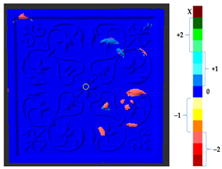
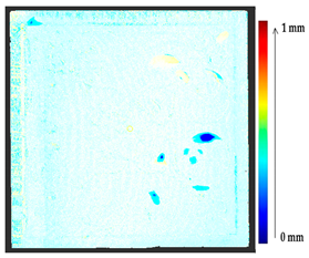
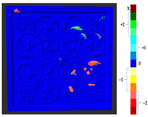
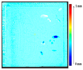
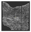
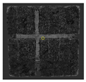
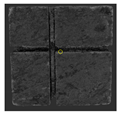
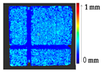
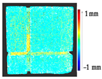
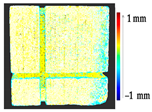
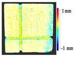
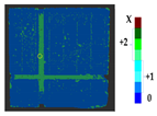
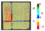
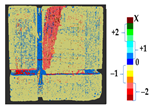
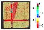
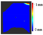
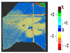
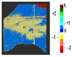
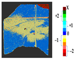
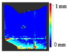
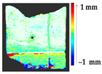
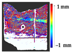
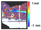
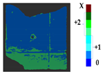
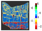
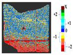
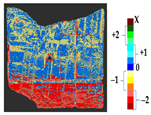
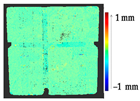
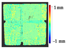
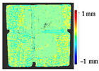
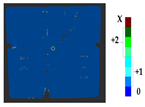
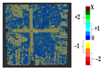
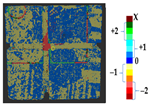
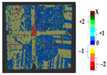
This work proposes a change-based segmentation method for applications to cultural heritage (CH) imaging to perform monitoring and assess changes at each surface point. It can be used as a support or component of the 3D sensors to analyze surface geometry changes. In this research, we proposed a new method to identify surface changes employing segmentation based on 3D geometrical data acquired at different time intervals. The geometrical comparison was performed by calculating point-to-point Euclidean distances for each pair of surface points between the target and source geometry models. Four other methods for local distance measurement were proposed and tested. In the segmentation method, we analyze the local histograms of the distances between the measuring points of the source and target models. Then the parameters of these histograms are determined, and predefined classes are assigned to target surface points. The proposed methodology was evaluated by considering two different case studies of restoration issues on CH surfaces and monitoring them over time. The results were presented with a colormap visualization for each category of the detected change in the analysis. The proposed segmentation method will help in the field of conservation and restoration for the documentation and quantification of geometrical surface change information. This analysis can help in decision-making for the assessment of damage and potential prevention of further damage, and the interpretation of measurement results.
1. Introduction
There are two main approaches to surface geometry segmentation: geometry (single geometry representation based) and change segmentation (two or more states represented by corresponding geometries). The single geometry segmentation implies the detection and grouping of similarly shaped objects’ parts, while change segmentation is the grouping of likewise change behavior parts of the data. The change analysis of data from surfaces on CH objects involves the comparison of two or more 3D geometries to assess the global statistical information [1,2]. This is essential to have a brief overview of the changes, which might be related to natural aging and deformation, as well as to surface alterations and the formation of crusts, purposeful destruction, or the addition/removal of material during restoration. This information can be assessed by simply comparing the two geometries and their different parameters. In Reference [3], the change detection was performed by using the global geometry comparison method of cloud to mesh (C2M), where they lost information while creating the mesh for the compared surface. Later a direct point-to-point geometry comparison was developed in Reference [4], which is a model-to-model cloud comparison (M3C2), and applied for change detection in References [1,5]. The method could identify the loss and deposit on the surface irrespective of noise and unsmooth region. These works were dedicated to CH change detection over time; however, they were conducted by using a physical marker for the reference. The use of a physical marker is prohibited for various CH objects. Moreover, the global geometry comparison alone is sensitive to the cross-time registration error of the two models. In our approach, we overcome the registration error based on the known unchanged part of the surface and use of physical marker for the change detection. However, it would be beneficial if the global change information could be identified and grouped based on the behavior of the change of local geometry of each point on the surface.
There are many approaches to segmentation and automation for one-phase geometry identification dedicated to CH [6,7,8], using several geometric rules. The scanning of real objects is affected by various problems that make it difficult to perform the segmentation without uncertainty. The common factors that produce ambiguity in the recognition process of classification are point location noise [9,10,11], mostly from the uneven part of the surface, the thermal noise of CCD/CMOS detectors, optical phenomena [12], and the coarse representation of continuous surfaces due to triangular approximations [13]. The most common approaches for the geometric segmentation process are edge-based (curvature), region-based (density, smoothness, similarity), model-based, and hybrid methods, where both edge-based and region-based segmentation are used [14]. The use of machine learning approaches makes the method more robust to the overall noise, as well as region noise and occlusions [7,10,11,15,16]. However, there is no required segmentation functionality defined in the application to CH change measurements. Change-based segmentation is an attempt to identify and classify the behavioral similarity of the change occurrence and assign it a linguistic attribute for a portion of the surface [17]. However, in the field of preservation and documentation of CH objects, information can be collected in various ways like 2D RGB, Multispectral Imaging, infrared, 3D information, Reflection Transformation Imaging or combining 3D with RGB or multispectral [18], according to the analysis needed and the selection of data accumulator, irrespective of the size of the data [5]. The change-based segmentation can be obtained from 3D scanning of an object’s surface and can be localized to detect and calculate surface geometry changes over the monitoring period [19]. To highlight gaps in knowledge, with specific reference to CH research, the analytical approaches of geometry segmentation are presented based on geometric analysis of an object’s surface in general 3D application fields. The study was performed on the previously developed one-phase geometry segmentation methods and tested to incorporate the same with our proposed segmentation dedicated to the change measurement in CH over time.
This paper proposes a novel change-based segmentation method of CH surfaces that could support 3D sensors with additional functionality. This method assesses changes between the target and source geometry models captured at different time intervals. It is based on analysis of the local distance’s histograms between the measuring points of the source and target models. Then the certain parameters of the histograms are determined, and predefined classes are assigned to target surface points. The overall data-processing chain is composed of four major processing stages, i.e., reconstruction of the 3D models, global and local geometry analysis, segmentation, and visualization. The analysis of the collected data and tracking down changes in CH objects over time (from different aspects, such as humidity, rainfall, snowfall, climate change, etc.) involves a set of problems for which the proposed method could provide detailed information on a 3D surface. In addition, it can help conservators and scientists in the documentation with the 3D digital representation involved in their work. The work is also focused on developing visualization of the results obtained on the surface to make it a more user-friendly representation of detected changes. The goal of the work is in line with the application of optical sensing techniques to CH, monitoring and grouping changes on the surface of CH objects before and after conservation.
2. Methodology
To further improve the digital documentation of change on CH objects, we propose a segmentation method to recognize the several different possible states of changes locally on the surface. The goal of this work is to develop an automated change-detection method to retrieve various behaviors of local geometry for each point change from the CH surface. To do this, we considered calculating the distances between each point from the target surface to the source surface. However, for that, accurate point-to-point mapping between the two stages of data is a crucial step to calculate the actual value of the change. In this work, a corresponding changed point search algorithm was developed in four stages, considering the direction of the normal vector of the target surface point and the displacement vector from the target to the source surface point. The Euclidian distance was calculated in four different ways, from each point on the target surface to the corresponding changed point on the source surface, to analyze its influence on the segmentation results. For each surface point, a local distance histogram was stored, and certain parameters were calculated. From the calculated parameters, the identification of each surface point was performed and stored in a separate category. Based on the expertise of the conservators, each detected category was inspected and named locally, based on the restoration/conservation and monitoring over time. In this work, we also considered developing the visualization of the results, i.e., a representation of colors for the types of change on the surface, to make it a more user-friendly representation of the detected changes, based on the histogram behavior. In this section, a detailed description of the four major phases of the entire work, as introduced above, is given.
2.1. Reconstruction
In this section, the 3D modeling of the object is composed of two phases, i.e., stitching of the filtered point clouds to reconstruct the 3D model and cross-time alignment of more than one model.
2.1.1. Stitching of Point Clouds
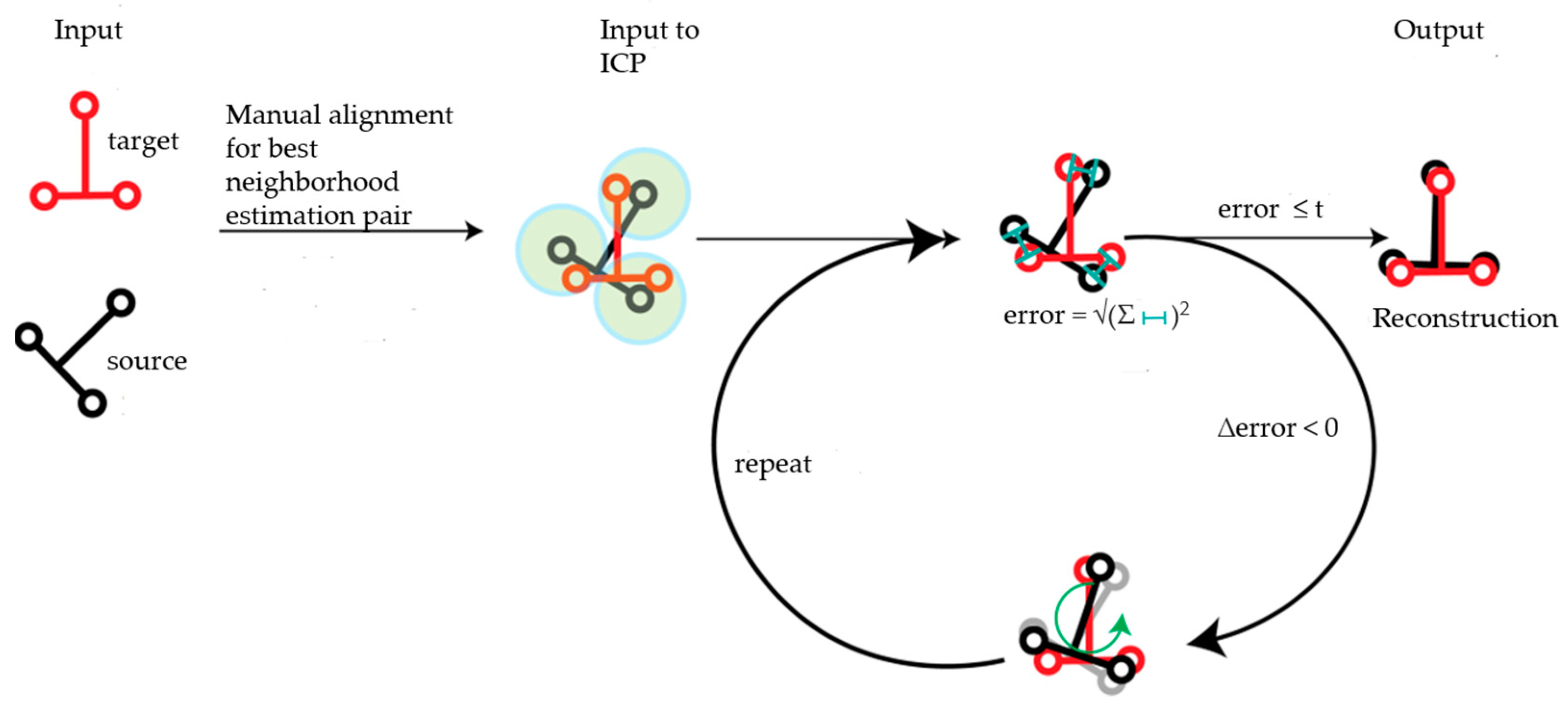
To reconstruct the 3D model for the selected object, each of the filtered point clouds was stitched together in the real coordinate space concerning a target point cloud (T0). For the rest of the source scans (T1… n), a manual alignment close to the target point cloud was introduced for a rough estimation of the 3D model of the object from the user perspective view. Then stitching of the scans was performed by using the optimized iterative closest point iteration (ICP) algorithm [20] for each pair of point clouds. ICP was recursively performed as shown in Figure 1 for each pair of consecutive point clouds until the minimum error of the algorithm was reached. A condition was set for the number of iterations to the best fit: the calculated root mean square (RMS) of the ICP algorithm ≤Threshold value (t). The average point-to-point distance of target was considered as the threshold value for this analysis. The global transformation induced in the source point cloud was stored to get the final 3D model of the entire object’s surface. For the next run, T1 was considered the target point cloud, and the source scans are updated as T2… n.
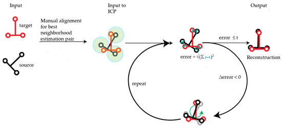
Figure 1.
Sketch of the reconstruction of the 3D model.
2.1.2. Cross-Time Alignment of the Models
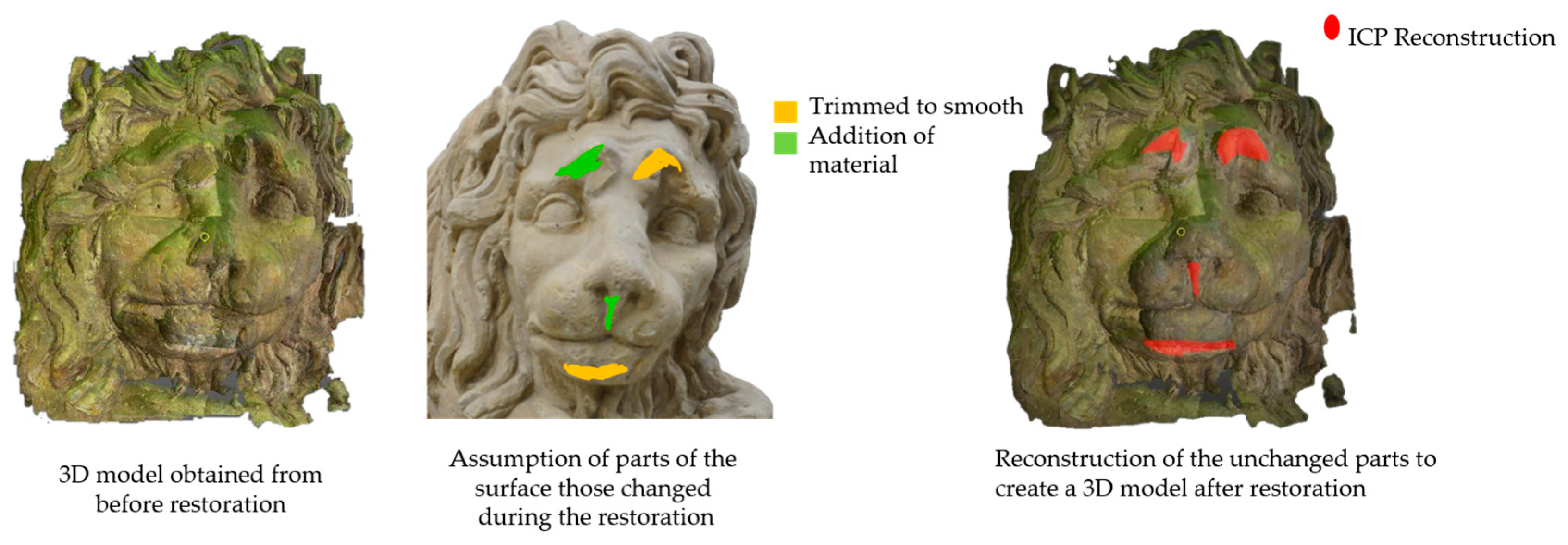
The cross-time alignment of the data from two different phases, i.e., before and after change, in terms of variation in size of the data is a global problem. However, to compare the geometry over time, the 3D models obtained from the two measurements of the same object must be aligned in the same 3D space. By following the same ICP algorithm, we can align the 3D models by considering each complete model as a single point cloud. However, in a real scenario, the alignment error is not accurate, which affects the quantification of surface geometry changes. In the case of restoration of an object, if the object has induced changes only on a known part of the surface, the alignment error influence can be minimized. After the initial ICP algorithm, a second pass can be performed, considering only the unchanged part of the surface, as shown in Figure 2. Later, calculated transformation could be applied to the whole changed surface model. This is only to avoid alignment error and confirm the correctness of the proposed geometry comparison method [21]. However, when the object has a change on the whole surface, especially concerning an outdoor monitoring or even the chemical treatment or cleaning of the object’s surface [22], having no reference to be considered as no change, the entire 3D model must be aligned by using the ICP algorithm. There is a small possibility of avoiding alignment error, even from the concerned monitoring period, based on the expertise of the conservation scientists: a certain time interval can be considered as involving no change for some object’s material.

Figure 2.
Three-dimensional model of the face of the ‘lying lion’; sandstone; 150 × 71 × 86 cm; owner: Radziwiłł Palace in Nieborów; possible solution to avoid alignment error for the face (~30 × 35 cm) in case of known reference of no change.
2.2. Global Geometry Analysis
In this section, the occurrence of surface changes was assessed by comparing both the target and source models obtained over time. After alignment of the models, the global change of the surface geometry over time was quantified. We calculated the changes in the geometry of the object for each surface point and its respective neighborhood points’ displacement behavior.
2.2.1. Point to Point Absolute Distance (P2P)
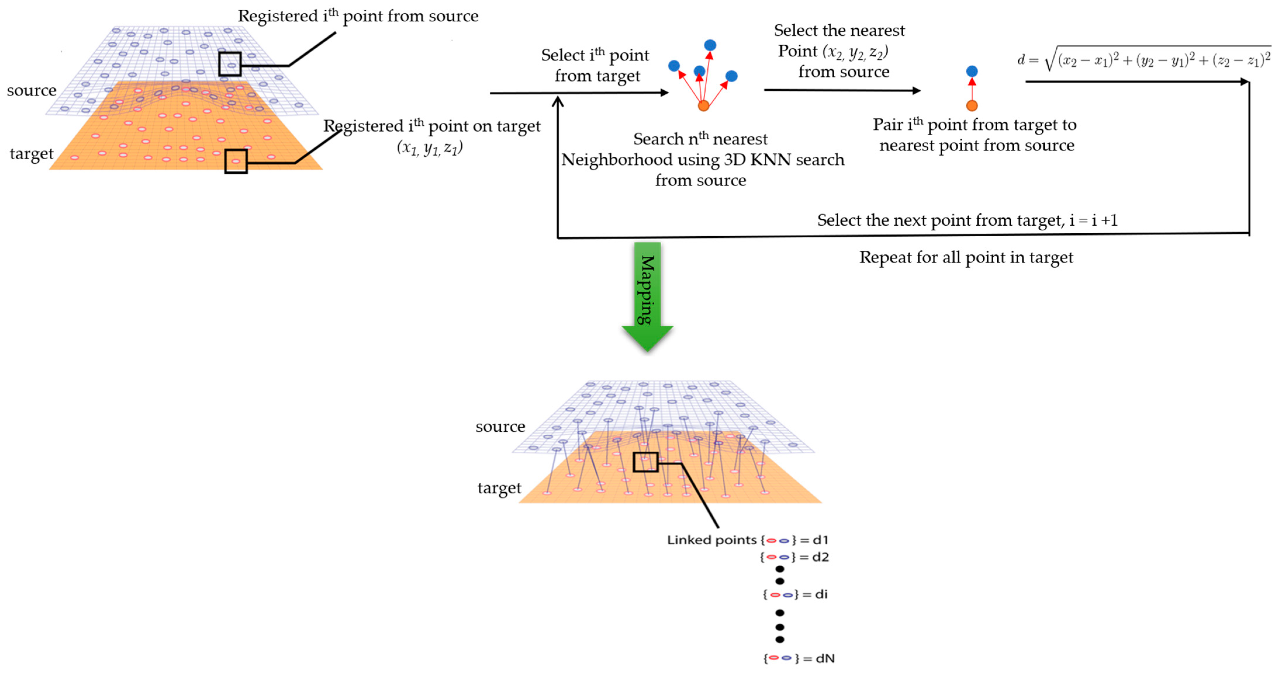
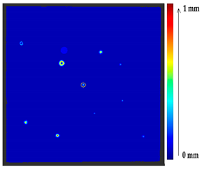
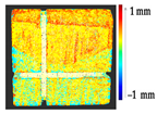
The comparison of the 3D models of the object was performed to assess the global change in the surface geometry. The analysis of the global change can help to identify roughly what changed on the surface. In this section, the absolute 3D distance from each surface point of the target to the nearest surface point on the source is calculated as shown in Figure 3. Based on the minimum and maximum values obtained, a color map is generated to represent the quantification of change on the target surface.

Figure 3.
Sketch of the P2P distance analysis.
2.2.2. Point-to-Point Vector Distance (P2P_Direction)
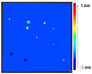
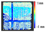
In the absolute distance calculation, the information was not clear enough regarding the direction of the change with respect to the target, as shown in Figure 4, with red (shifted up) and black (shifted down) arrows. Additionally, in the analysis, the conservators were interested to see whether the surface points are going up (deposit) or down (material loss).

Figure 4.
Direction of change distance calculation.
In the direction distance analysis, the dot product of the normal vector (n) of each point on target was computed with the displacement vector (d) to each nearest point on the source. The normal vectors were calculated for each surface point of the target, creating a neighboring plane among its neighbor points, towards the direction to the 3D scanner for the necessary measurement device. The dot product between the two vectors gave a sign information to the change, considering the target as a reference of the change. The direction of change is an important factor that helps us to analyze the change in the surface to identify the surface points and whether it is a loss or a deposit. However, in the case of a known restoration process where gap filling is performed [21], P2P absolute distance calculation will work efficiently.
2.2.3. Point-to-Point along Normal Vector (P2P_AlongNV)
In the above distance calculation method, the consideration of the nearest point may not always correspond to the actual change point on the source, especially when it comes to the unsmooth and curvy parts of the surface. A scenario is presented in Figure 5. The consideration of the nearest point will work if the surface changes linearly, as shown in Figure 5a, but in Figure 5b, it will not correspond to the actual change point to the target. In the figure, the consideration of the changed point is shown with a green arrow and the actual changed point is shown with red arrow in Figure 5c.

Figure 5.
Scenarios (a). Smooth (b). Non smooth and (c). Actual of finding the corresponding changed point from target to source.
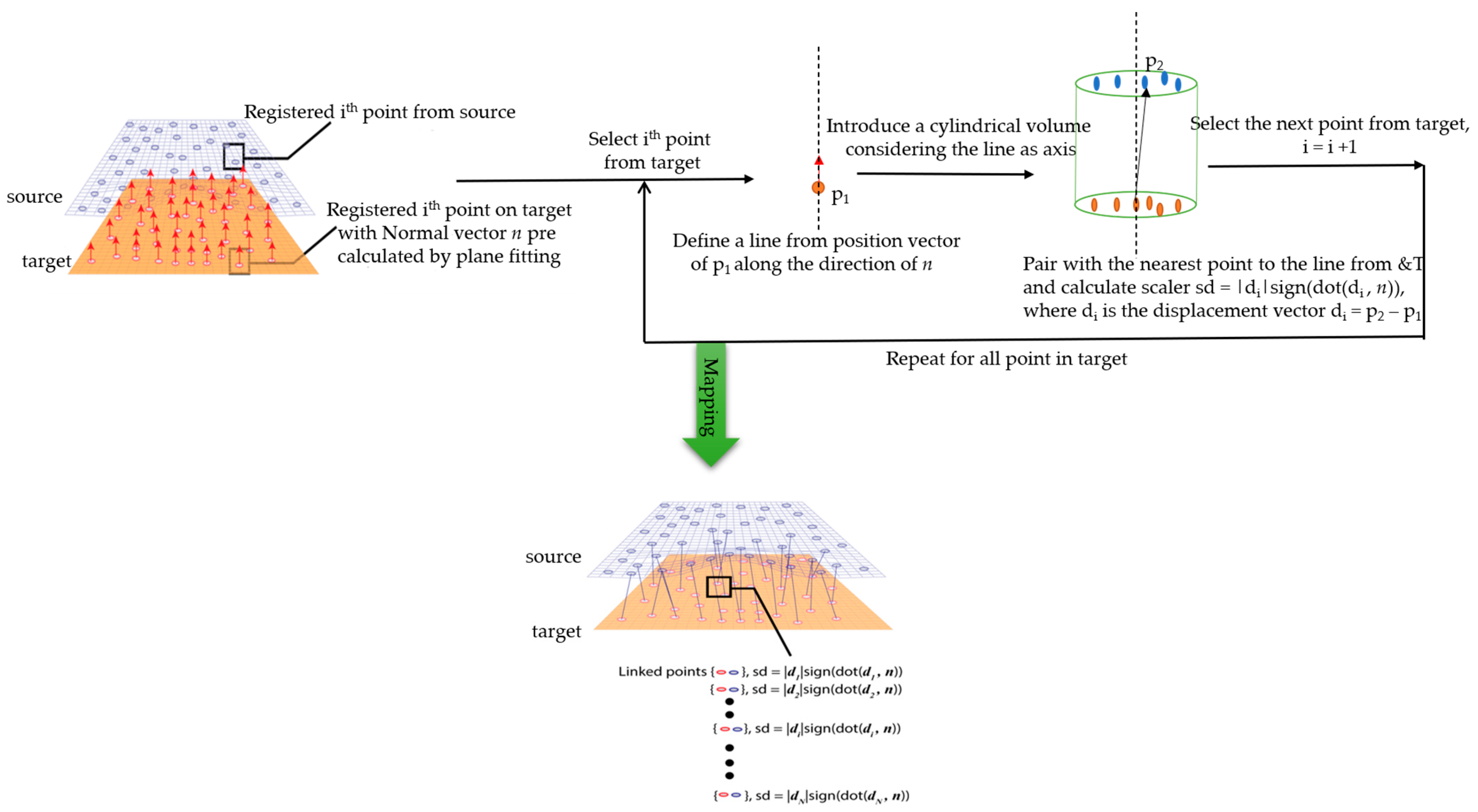
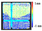
To avoid the corresponding change point consideration, in the analysis, a strategy was adopted whereby the corresponding change point was considered along the normal vector of the selected point on target to source. A line was drawn along the direction of the normal vector via the selected point from target, and the distance was computed within a specified cylindrical volume on source to the line. The nearest point to the line was considered as the corresponding changed point from source for each selected point on target. After finding the corresponding nearest point to source, the displacement vector was computed with the normal vector of target model. To optimize the search for a nearest point to the line, a user-defined radius was set. The working principle for the P2P_AlongNV distance calculation method is shown in Figure 6. The search will retrieve a zero value if the nearest point cannot be found within the specified region. In this case, when the search retrieves a value of zero, either the search radius can be increased for those points, or it can be presented as zero if it cannot find a point after the increase in the search radius.
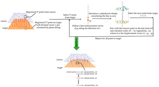
Figure 6.
Sketch of the P2P_AlongNV distance calculation.
2.2.4. Point-To-Point Projection along Normal Vector (P2P_ProjectionAlongNV)
In this section, the P2P_AlongNV was slightly modified by projecting the considered nearest point to the line along the normal vector, as shown in Figure 7. The corresponding change point was considered on the line, and the displacement vector was computed from the normal vector to quantify the change and its direction with respect to the target.
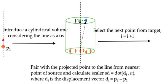
Figure 7.
Sketch of the P2P_ProjectionAlongNV distance calculation.
2.3. Local Geometry Analysis
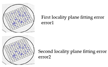
The local geometry analysis is based on the optimized k-neighborhood points and computing the distances of four types, as mentioned above, with the source for each point on target. For each point on target, the nearest point was computed up to a radius (r) of the scaled average point-to-point distance of source, with consideration of the local neighborhood change analysis. The local distribution as shown in Figure 8 is the basis for a further analysis of the change information locally and grouping the data based on the similarity of their behavior.
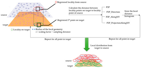
Figure 8.
Sketch of the local neighborhood distance analysis.
2.4. Segmentation
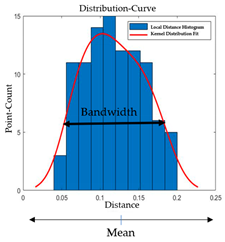
In this section, a change-based segmentation is proposed to train the method to automatically detect the types of changes that occurs on the surface over time. The respective distances of the k-neighborhood points were calculated for each point on the target model and stored as the local distance behavior in histograms. Then, using the calculated local neighborhood histograms for each point, the calculated data were fit to the kernel distribution curve [23]. As the fluctuation of the local neighborhood distance histogram produced by the data is very irregular, the random and discrete kernel distribution can sum up the component smoothing functions for each data value to produce a smooth, continuous probability curve [24,25].
The estimation of kernel density function, fn, for given n number of points with density, f, is defined as below:
here K and h represent the kernel function and the smoothing parameter or window width, respectively.
In Equation (1), the value of the window width, h, can be set by using Silverman’s (1986) recommendation [26], which uses a default width of the DATA PLOT as follows:
In Equation (2), s is the sample standard deviation, and IQR is the sample interquartile range.
The selection of the optimal window width depends on the underlying estimated function, and it works reasonably good for a wide variety of distribution.
The analysis showed that the local neighborhood distance histograms obtained are normally distributed in this work. Since the underlying data are normally distributed according to Silverman’s DATA PLOT, the optimal width is calculated as follows:
where n is the number of points in the raw data, and s is the sample standard deviation of the raw data.
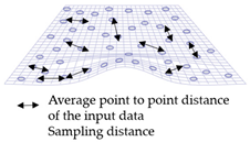
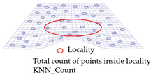
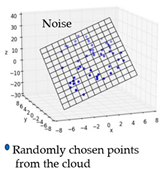
In the proposed approach, several parameters were considered, with the calculated local distance histogram as an input to the segmentation method, as shown in Table 1. Moreover, several user-input threshold values were incorporated into the segmentation method, as shown in Table 2, to make the grouping based on the 3D model fitting and quantitative analysis of the amount of change based on the size of the object. The bandwidth for each category of change segmentation was assigned based on the sampling distance and noise obtained at each of the point clouds from both stages of data. However, in a real scenario, as mentioned in Section 1, the data collected from CH surfaces are not structured and supervised. They also contain thermal noise from the detector of the 3D scanner detector. To overcome the noise from the surface and make the method insensitive to noisy data, the surface noise was parametrized, and conditions were set based on the obtained histogram parameters.

Table 1.
Considered input parameters to the segmentation method.

Table 2.
User input thresholds to the segmentation method.
The conditions were set to the parameters considered in Table 1 and Table 2 for change-based segmentation.
The parameters were defined for the analysis, as in Table 3.

Table 3.
Ground truth based on the histogram parameters.
2.5. Visualization
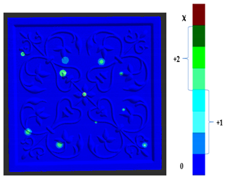
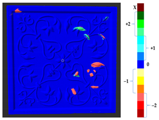
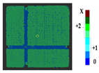
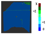
To represent the results, after grouping the surface points with the respective type of change, a color map was generated on the target point cloud to represent the same on the surface. In the visualization section, the colors for each change type were specified and we set the colors to the target model to make it an easier and more user-friendly application. In the analysis, the colors chosen for each identified change were assigned, as shown in Table 4. The visualization on the surface is presented in the tables, with obtained results from the segmentation method for each type of change mentioned in Table 3. An exemplary model, as described in Figure 2, is presented in Figure 9, and identified changes are shown on the surface with the specific colors for each category of change.

Table 4.
Assigned color code and number for each category of change.
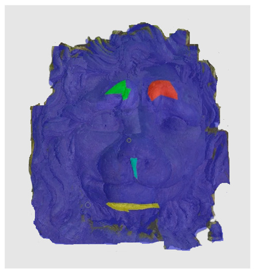
Figure 9.
Exemplary visualization of detected changes on the surface for object originated from Figure 2.
3. Results and Analysis
Two case studies were considered for the analysis. For Case Study I, the data were collected by using a structured light-based custom-designed 3D scanner [27] developed at the Faculty of Mechatronics at Warsaw University of Technology, Poland. This device has a maximum permissible error of 0.25 mm. For Case Study II, the 3D datasets considered were from the PRESIOUS project [28]. The postprocessing of the data for the proposed method was written in FRAMES, which was also developed at the Faculty of Mechatronics, Warsaw University of Technology, Poland, and written in C++ [29].
3.1. Case Study I
3.1.1. Results of Simulated Data
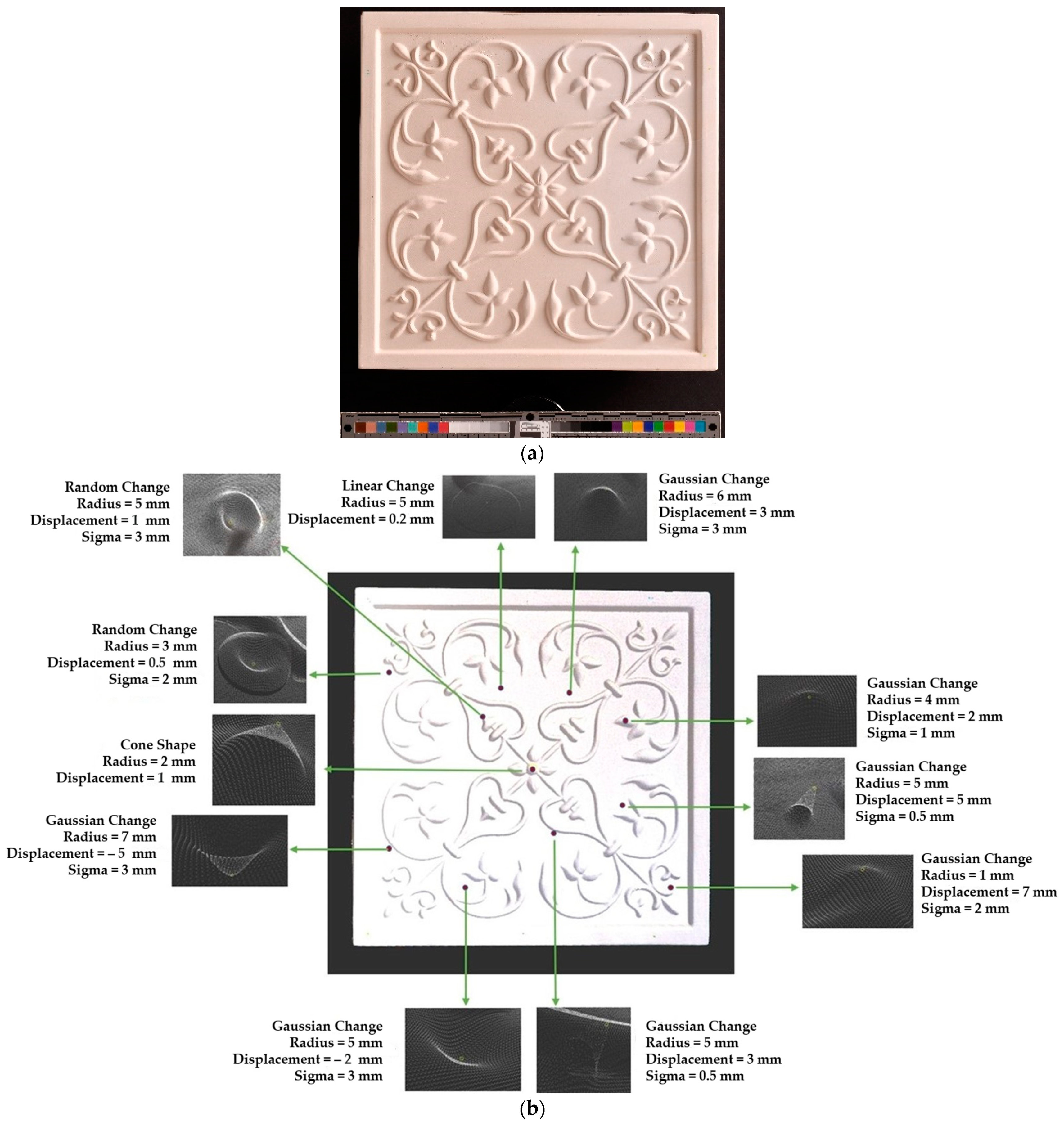
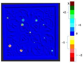
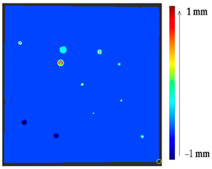
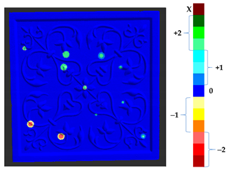
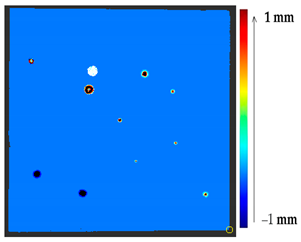
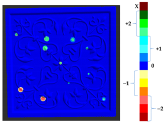
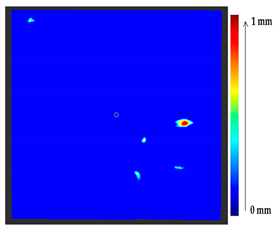
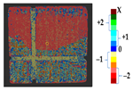
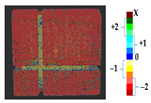
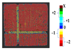
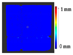
To verify the appropriateness of the proposed segmentation method, a mock-up of a ceramic tile of size 220 × 220 × 45 mm3 for a tile stove was prepared by a group of restorers, as shown in Figure 10a. The approximate depth of relief of the tile was 4 mm. The original state of the model was scanned to obtain the target model. The captured data were filtered out from the outliers and external noise based on a Hausdroff distance calculation, and we removed faraway points based on a threshold input distance. The complete model was obtained after stitching each point cloud, using the ICP algorithm. At the beginning of the analysis, to assess the ground truth of Table 3 and avoid cross-time alignment error, several manual changes were made with known values on the original surface. The changes were introduced on the surface points to prepare the source model as shown in Figure 10b, and the obtained results with the input parameters as shown in Table 5 are shown in Table 6.

Figure 10.
Tile reconstruction; ceramic; 220 × 220 × 45 mm. Owner: Academy of Fine Arts in Warsaw, Poland. (a) Original state of the tile and (b) changes introduced manually to the original surface.

Table 5.
Calculated and user input parameters for Case Study I.

Table 6.
Correctness of the ground truth table.
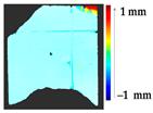
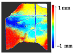
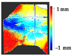
The results from the simulated surface, as shown in Table 6, for the proposed method, and specifically from the global geometry analysis of P2P, the negative and positive displacement cannot be predicted. However in the P2P_Direction, P2P_AlongNV, and P2P_ProjectionAlongNV global distance calculation, the direction of change is detectable. And from the segmentation analysis, the locations of the changes made and their impact on its local geometry were detected more clearly. In this case study, the segmentation approach of four different distance calculations did not show much difference, as the manual changes were made precisely and smoothly on selected points.
3.1.2. Results of Real Scenario
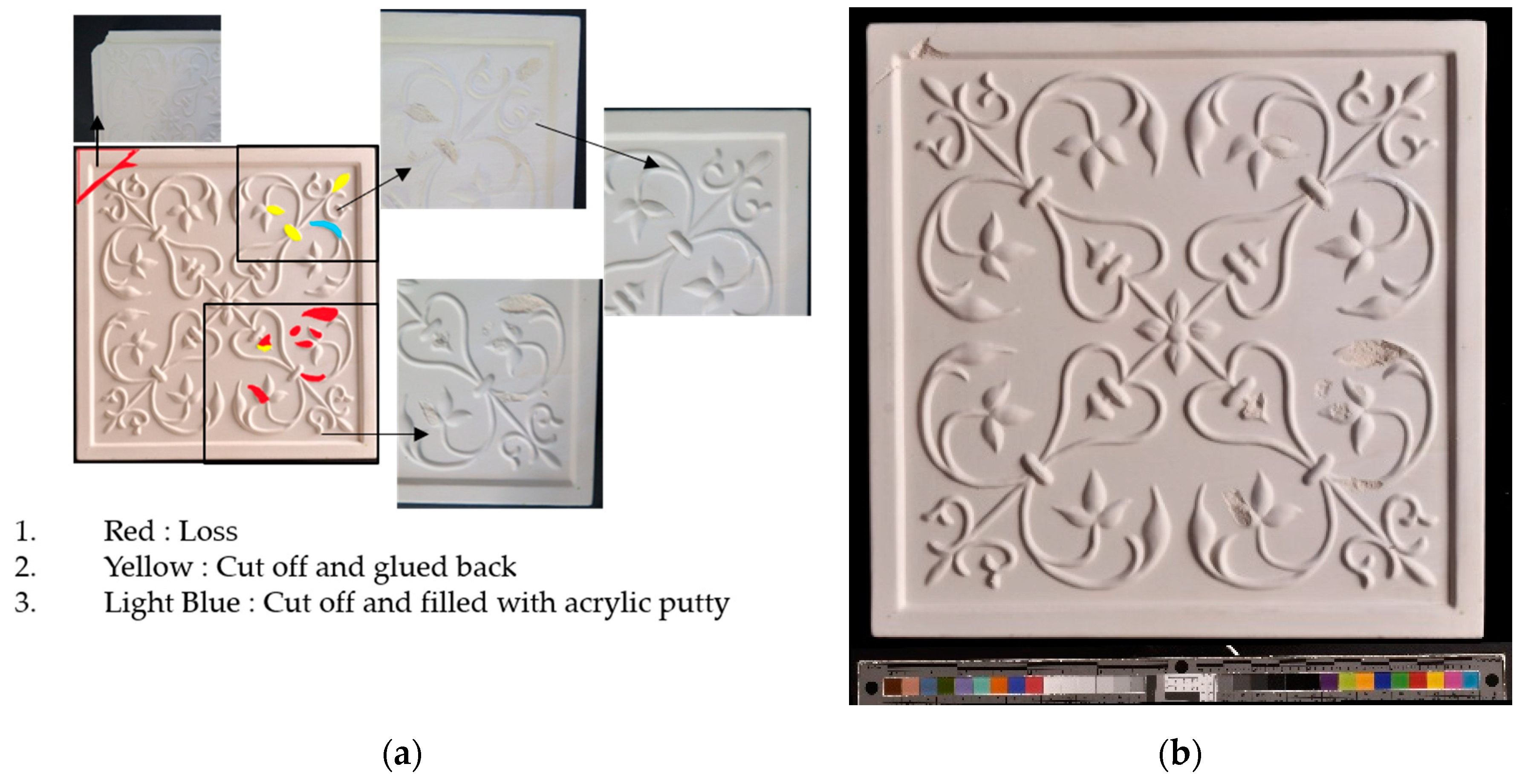
A tile was considered to represent the restoration problems encountered with sculptures and other ceramics. Several changes were introduced to the tile, such as loss, gluing, displacement of the decorations, gluing of a large piece of the object, and gap gilling with acrylic putty to achieve the reconstruction of the tile, as shown in Figure 11a. The original state of the tile is shown in Figure 10a. Figure 11b shows the outcome after the mechanical changes were made on the tile.
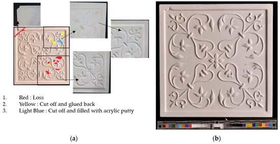
Figure 11.
(a) Changes made to the tile; (b) the changed tile.
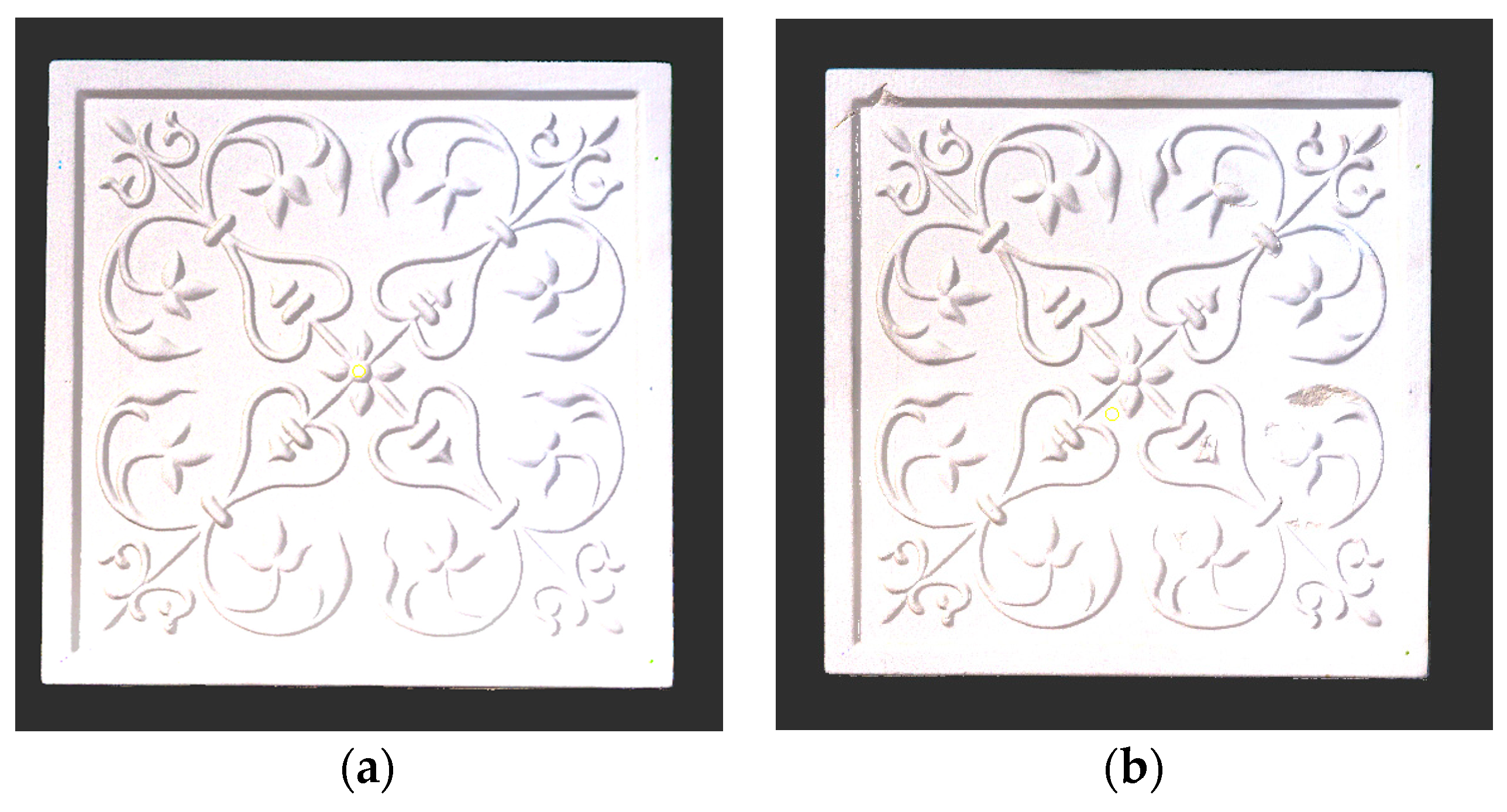
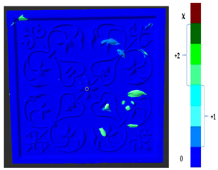
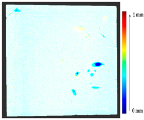
For a quantification of the induced change in the real scenario, the analysis had to register both the target and source models in one time frame, using the ICP algorithm mentioned in Section 3.1.1. To overcome the alignment error and places of changes made along with the noise, the Nonchanged Threshold (Nt) described in Table 2, with reference to the unchanged part of the surface, was set. The input parameters to the segmentation method were set as shown in Table 5. The models obtained before and after are shown in Figure 12 and the calculated results are presented in Table 7.
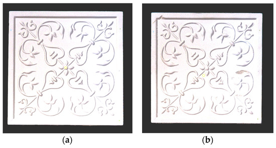
Figure 12.
Three-dimensional models of the original surface (a) and changed surface (b) of Case Study I.

Table 7.
Correctness of the ground truth table with Nonchanged Threshold.
The results from the ceramic tile were verified by a group of restorers and the correctness of the method was justified via the locations of damage and displacement on the surface, which could not be detected in a global geometry analysis. The results showed a loss of more than 2 mm of material where parts of the surface were damaged. In the analysis, we detected the misalignment of gluing as a deposit of less than 0.5 mm to the surface, indicating that, while gluing back the parts, they were not placed properly, or the thickness of glue caused the displacement of the decorations. The part of the surface that was filled with acrylic putty showed a displacement on the surface as the filling was slightly tilted in relation to the original shape. Moreover, during the removal of a corner of the tile for investigation reasons, a very small part of the ceramic was lost. The gluing was performed correctly, but the loss was not filled with putty; this part was recorded during the scanning process and noted as a loss in the analysis. The method can be claimed as correct in cases when a part of the surface remained unchanged, and the user can consider it as a reference to set the threshold Nt. However, this practice is not suitable with an increase in the threshold Nt, as this would result in losing some information due to both the minor deposit and the loss.
3.2. Case Study II
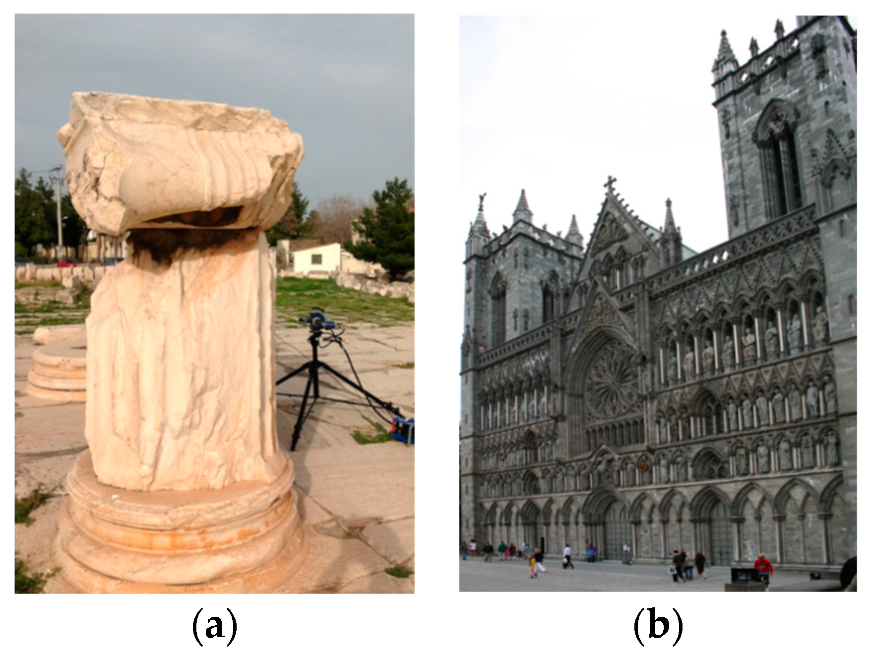
The second case study considered monitoring over time. Several datasets were considered to test the method from the PRESIOUS project [28]. The monument sites that were studied during the project work are shown in Figure 13.

Figure 13.
The two CH monuments considered for study: (a) The Sanctuary of Demeter and (b) Nidaros Cathedral in Trondheim, Norway.
Several datasets were considered for the analysis, as shown in Table 8, from two sessions. During the project work, stone slabs were used for accelerated erosion experiments with the treatment of various chemicals and monitored over time.

Table 8.
Stone-slab labeling and two chosen sessions of data collection.
The results show the erosion and loss of material from the stone slabs over time. The 3D models for Case Study II were obtained, as shown in Table 9, from the PRESIOUS project. Two different time interval models were registered in one time frame, using the ICP algorithm.

Table 9.
Three-dimensional models of the considered stone slabs from two different times.
The analysis was carried out on each considered dataset with two different time measurement to assess the changes that occurred during the erosion process, with the values of parameters shown in Table 10. The results and a detailed discussion of the changes from chemical reactions (see Appendix A) are provided below. The calculated results obtained from the analysis and the corresponding surface point count information for each considered datasets are shown in Table 11, Table 12, Table 13, Table 14, Table 15, Table 16, Table 17, Table 18, Table 19, Table 20, Table 21 and Table 22.

Table 10.
Calculated and user input parameters for Case Study II.

Table 11.
Analysis and results for the dataset of EL3.

Table 12.
Analysis of surface points count on the surface of EL3.

Table 13.
Analysis and results for the dataset of ES1.

Table 14.
Analysis of surface points count on the surface of ES1.

Table 15.
Analysis and results for the dataset of NGL2.

Table 16.
Analysis of surface points count on the surface of NGL2.

Table 17.
Analysis and results for the dataset of NBL1.

Table 18.
Analysis of surface points count on the surface of NBL1.

Table 19.
Analysis and results for the dataset of NBL2.

Table 20.
Analysis of surface points count on the surface of NBL2.

Table 21.
Analysis and results for the dataset of NGS1.

Table 22.
Analysis of surface points count on the surface of NGS1.
It is difficult in an actual case study to determine which parts of the surface undergo no change or a minor deposit and loss as during the monitoring period there are no physical markers used as a reference. In this case study, the Nonchanged Threshold could not be increased as the part of the surface that remains unchanged over time was unknown. In addition, the mass loss and mean erosion calculations showed that the Nidaros Bad stones underwent a greater loss compared to Nidaros Good and Marble, and the same can be seen in the proposed analysis. Additionally, the point count analysis to measure the surface area with loss and deposit showed that Nidaros Bad stone slabs had a loss on a greater part of the surface compared to Nidaros Good. However, the marble slabs also showed a loss on a greater part of the surface, yet the quantification of loss was smaller than for Nidaros Good. The datasets of Nidaros Bad showed a total loss of material from the surface, as shown in Table 17 and Table 19. Nidaros Good showed more loss than the marble stone slabs. The analysis can be easily interpreted and claimed to be correct for any mechanical changes during the restoration process. However, in real-case monitoring, such as chemical weathering or physical/mechanical weathering, as performed in the PRESIOUS project, these are unpredictable.
4. Conclusions
In this work, an analysis method with two or more change stages for 3D geometrical data was developed. The 3D analysis of geometrical changes was performed by comparing the local geometry of two phases of surface information. This provides information about the behavior of geometry changes and segments the surface into areas with similar characteristics. The computational analysis of each surface point and its respective neighboring points’ behavior can provide the local geometry changes, comparing more than one phase of data and leading to a better understanding of the changes over time on CH surfaces.
In the distance calculation, the focus was on direct comparison of each surface point rather than meshing the surface to assess the direction of change. The P2P computation method provides an overall good visualization of the change parts on the surface failing to provide information about the direction of change. The P2P_Direction method works well in smooth and slightly eroded surfaces, providing the change direction as on the simulated surface for Case Study I, whereas the P2P_ProjectionAlongNV showed a promising result, providing more information irrespective of the surface smoothness and noisy data. The P2P_AlongNV method computes for a local distance between the two points along the normal vector direction but fails when the corresponding change point is far away from the line along the normal vector. The P2P_ProjectionAlongNV method provides additional projection confidence for each computation of the corresponding change point along the normal vector line providing better region segmentation. However, for simple deformations (in Case Study I), the P2P_Direction method provided an acceptable result, but showed a minor deposit where gluing was performed, whereas the P2P_AlongNV and P2P_ProjectionALongNV showed major deposits with the same value of deposit threshold, which agrees with the expectations. The P2P_AlongNV and P2P_ProjectionALongNV methods better quantified the change as P2P and P2P_Direction consider the immediate neighboring point from the compared dataset as a corresponding change point. For Case Study II, for the datasets of NGL2, NBL1, and NBL2, as shown in Table 15, Table 17, and Table 19, the distance calculation method P2P_ProjectionAlongNV provided more information about the major material loss with a better visualization. To sum up, the P2P_ProjectionAlongNV method allows for the visualization of changes most in line with the expectations of art conservators and is recommended for the assessment of changes in the surface of cultural heritage objects.
However, the proposed method is sensitive to the initial cross-time alignment of consecutive datasets. The aim of this work was to assess and classify the changes of surface geometry of CH objects from two-time intervals. However, the cross-alignment of the two models is an open issue when the entire surface has a change over time. In the analysis, we tried to solve the alignment issue up to a certain point by introducing the Nonchanged Threshold, but it is hard to claim the same when changes occur on the entire surface and there is no reference point with no change. The results should help improve the 3D documentation of the quantification of surface changes of CH objects over time. The analysis and its correctness were more promising in Case Study I than Case Study II, due to the lack of a reference with no change. The proposed analysis and grouping method could help lay users or conservators to analyze and present their work more clearly during restoration. The analysis can access the details of each surface point’s behavior and show how it is changing over time. The method is automated and insensitive to the noise of the input data. The user can set the threshold value of deposit, loss, and alignment based on the registration and easily access the surface change information. The colormap visualization of each change category makes the proposed method very convenient and user-friendly. This analysis is not limited in terms of the composition or size of the object, thus making the method more flexible and reliable.
In this paper, the measurement was performed on surface geometry change segmentation. However, displacement or deformation of material, changes in the shininess of a CH surface, color, or spectral information changes should be taken into consideration. This work can be extended to multimodal image data. The proposed analysis will be helpful for tracking down changes of surface texture, displacement, and color information over time. In the future, this segmentation approach will be tested on multimodal image data, considering reflectance imaging transformation, digital image correlation, and multispectral imaging.
Author Contributions
Conceptualization, S.S. and R.S. methodology, S.S. and R.S.; software, S.S and R.S.; validation, R.S., J.M. and N.L.W.S.; formal analysis, S.S.; investigation, S.S. and R.S.; resources, S.S.; data curation, S.S., and J.M.; writing—original draft preparation, S.S.; writing—review and editing, R.S. and N.L.W.S.; visualization, S.S.; supervision, R.S.; project administration, R.S.; funding acquisition, R.S. All authors have read and agreed to the published version of the manuscript.
Funding
This research has received funding from the European Union’s Horizon 2020 research and innovation program under the Marie Skłodowska-Curie grant no. 813789.
Institutional Review Board Statement
Not applicable.
Informed Consent Statement
Not applicable.
Data Availability Statement
The data used for this study will be made public at the end of the project via CHANGE-ITN project website and its data repository and can be accessed on request.
Acknowledgments
This work was carried out as part of the CHANGE (Cultural Heritage Analysis for New Generation) project of Warsaw University of Technology, Poland, supported and funded by the European Union’s Horizon 2020 research and innovation program under the Marie Skłodowska-Curie grant no. 813789. Our sincere thanks go to the PRESIOUS project (European Union’s Seventh Framework Program for research, technological development, and demonstration under grant no. 600533) for giving access to the datasets [28] used in this work. The financial support through the project granted by the Scientific Council of the Discipline Mechanical Engineering, WUT, is greatly appreciated. We would also like to acknowledge Radziwiłł Palace in Nieborów and Romantic Park in Arkadia/Division of the National Museum in Warsaw, Poland; Studio of Conservation and Restoration of Ceramics, Faculty of Conservation and Restoration of Works of Art, Academy of Fine Arts, Warsaw, Poland, for being great collaborators, providing invaluable suggestions, giving access to CH objects to work on, verifying the obtained results, and clarifying the proposed method as a tool for change detection.
Conflicts of Interest
The authors declare no conflict of interest.
Appendix A
The documentation during the PRESIOUS work (Figure A1) and a calculation of the mass loss and mean erosion helped confirm the correctness up to a certain point, considering the alignment error. This analysis shows the loss and deposit on the stone’s surface due to several chemical phenomena.

Figure A1.
Modeling an erosion process on the surface of a stone.
Figure A1.
Modeling an erosion process on the surface of a stone.
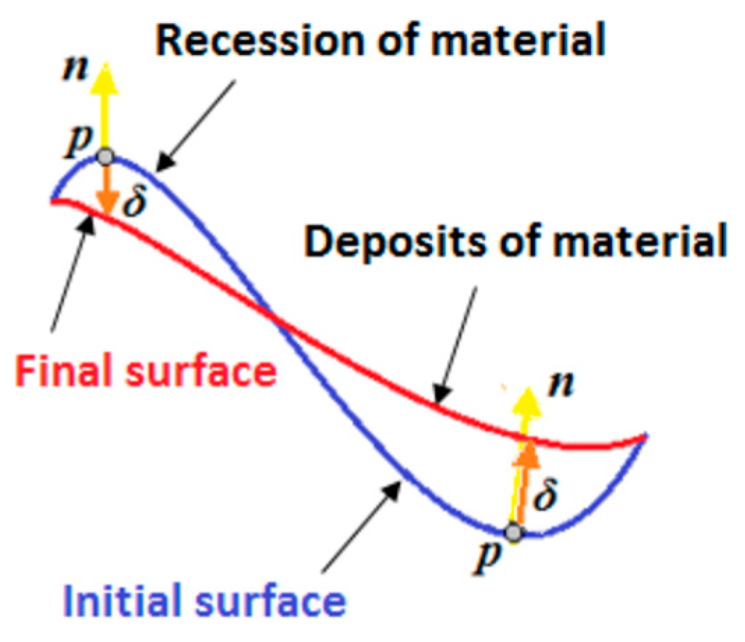

Table A1.
Stone slab material and associated experiments.
Table A1.
Stone slab material and associated experiments.
| Considered Stone Slabs for the Analysis | ||
|---|---|---|
| Stone Slabs | Material | Experiment |
| EL3 | Pentelic Marble | H2SO4 + HNO3(aq) Acid |
| ES1 | Pentelic Marble | H2SO4(aq) Acid |
| NGL2 | Grytdal Soapstone | Salt |
| NBL1 | Grytdal Soapstone | Freeze-Thaw |
| NBL2 | Grytdal Soapstone | Salt |
| NGS1 | Grytdal Soapstone | Outdoors/Trondheim |
The acidic treatment performed during the project work on the slabs of EL3 and ES1 (marble) led to them undergoing a chemical reaction on the surface. During this chemical reaction with sulfuric acid (H2SO4), a crystallized gypsum formed on the surface, as shown below:
CaCO3+H2SO4 → CaSO4 + CO2 + H2O
CaSO4 + H2O → CaSO4 · 2H2O
The formation of gypsum, which crystallizes as a dihydrous gypsum that is 150 times better (2.1 g/L) than a salt, such as CaCO3, on the surface would appear as a deposit on the surface during the geometry analysis. The formation of crystalline gypsum CaSO4·2H2O during the acidic treatment can cause destruction of marble due to bigger volume of gypsum by 100% than CaCO3, and it can show a deposit for a certain period but may also show as a loss from the surface after some point [30].
The compound formed during the treatment with nitric acid (CaCO3) is characterized by a very high solubility, as follows:
CaCO3 + 2HNO3 → Ca (NO3)2 + CO2 + H2O
Due to the low solubility of calcium salts, nitrates are washed away by rainwater or migrates to the stone as a solution where it enters to the decomposition process which may cause in loss of marble mass.
A strong acid treatment, such as H2SO4 and HNO3, on the surface of the soapstone might absorb water due to its higher porosity and lead to a crack/hole and then a part falling off from the edges or weak parts of the stone slabs. However, it is very hard to draw conclusions about the change behavior of the chemical treatment on the stone slabs due to insufficient information. From a restorer’s point of view, it is good practice to keep a reference point for making calculations of deposit and loss. Moreover, it must be kept in mind at which stage of the destruction phase the investigation started. The time interval chosen for monitoring might not be proper to investigate some interesting changes for conservation studies and make preventive restoration decisions.
The freeze-and-thaw treatment performed on the soapstone (NBL1), which was performed at −5 °C, resulted in a crystalline form of ice. Ice, having a larger volume, exerts a pressure of 0.6 MPa at the chosen temperature [30]. The capillary crack on the corner of the stone slab of NBL1, as recorded during the first session of scanning, might get filled up with water. This capillary crack is more prone to the action of ice, which can cause a total loss from the edges of the stone slab. However, for this treatment, there was also no reference point of unchanged surface, as the freezing must be performed on the entire stone slab.
The monitoring of the outdoor environment on NGS1 reflects the consideration of several environmental factors, such as the action of changes in temperature, humidity, pressure, and changes in the climate of location from where the object belongs to. These external factors can lead to the disintegration of the stones into smaller particles during the monitoring period. This kind of monitoring loses the reference of the unchanged surface, leading to unpredictable changes in terms of loss/deposit.

Table A2.
Changes in terms of mass of the selected stone slabs.
Table A2.
Changes in terms of mass of the selected stone slabs.
| Stone Slabs | m1 (g) | m2 (g) | Δm (g) | Δm/m (%) |
|---|---|---|---|---|
| EL3 | 27.5131 | 27.4734 | −0.0397 | −0.14 |
| ES1 | 27.5872 | 27.5156 | −0.0716 | −0.26 |
| NGL2 | 160.5487 | 159.4037 | −1.1450 | −0.71 |
| NBL1 | 168.8975 | Unknown | ||
| NBL2 | 188.9025 | 179.8329 | −9.0696 | −4.80 |
| NGS1 | 20.6227 | 20.5998 | −0.0229 | −0.11 |
Mass measurements during the project work showed that the stone slabs suffered from erosion under the specific experimental conditions of chemical treatment, in the following order:
Marble ≈ Nidaros Good < Nidaros Bad
The salt effect (NGL2 and NBL2) was shown to be more dramatic than the freeze–thaw effects, which were quite close to the acidic effects, and Nidaros Bad was the most sensitive stone type. Table A3 gives estimations of erosion δ by volume and surface area computations: (a) cubic approximation and (b) surface area approximation; and V1 initial volume (session 1) and V2 initial volume (session 2) of the accelerated erosion period are presented.

Table A3.
Estimated erosion by volume and surface area computation of the selected stone slabs.
Table A3.
Estimated erosion by volume and surface area computation of the selected stone slabs.
| Mean Erosion δ (mm) during Session 1 to Session 2 | ||||||
|---|---|---|---|---|---|---|
| Stone Slabs | V1 (cm3) | V2 (cm3) | ΔV (cm3) | S (cm2) | δ(a) (mm) | δ(b) (mm) |
| EL3 | 10.1391 | 10.1575 | 0.0184 | 29.7689 | 0.0065 | 0.0062 |
| ES1 | 10.1510 | 10.1497 | −0.0013 | 29.9718 | −0.0005 | −0.0004 |
| NGL2 | 55.2833 | 55.1410 | −0.1423 | 102.5810 | −0.0164 | −0.0139 |
| NBL1 | 61.7922 | Unknown | ||||
| NBL2 | 68.6979 | 66.6648 | −2.0331 | 125.6727 | −0.2040 | −0.1618 |
| NGS1 | 7.1294 | 7.1398 | 0.0104 | 24.6578 | 0.0047 | 0.0042 |
References
- Dante, A. Built-Heritage Multi-temporal Monitoring through Photogrammetry and 2D/3D Change Detection Algorithms. Stud. Conserv. 2019, 64, 423–434. [Google Scholar] [CrossRef]
- Logothetis, S.; Delinasiou, A.; Stylianidis, E. Building Information Modelling for Cultural Heritage: A review. ISPRS Ann. Photogramm. Remote. Sens. Spat. Inf. Sci. 2015, II-5/W3, 177–183. [Google Scholar] [CrossRef] [Green Version]
- Sitnik, R.; Lech, K.; Bunsch, E.; Michoński, J. Monitoring surface degradation process by 3D structured light scanning. In Proceedings of the SPIE 11058, Optics for Arts, Architecture, and Archaeology VII, Munich, Germany, 12 July 2019; p. 1105811. [Google Scholar] [CrossRef]
- Lague, D.; Brodu, N.; Leroux, J. Accurate 3D comparison of complex topography with terrestrial laser scanner: Application to the Rangitikei canyon (N-Z). ISPRS P&RS 2013, 82, 10–26. [Google Scholar] [CrossRef] [Green Version]
- Nicola, L. Monitoring earthen archaeological heritage using multi-temporal terrestrial laser scanning and surface change detection. J. Cult. Herit. 2019, 39, 152–165. [Google Scholar]
- Grilli, E.; Remondino, F. Classification of 3D Digital Heritage. Remote. Sens. 2019, 11, 847. [Google Scholar] [CrossRef] [Green Version]
- Murtiyoso, A.; Grussenmeyer, P. Automatic Heritage Building Point Cloud Segmentation and Classification Using Geometrical Rules. Int. Arch. Photogramm. Remote. Sens. Spat. Inf. Sci 2019, XLII-2/W15, 821–827. [Google Scholar] [CrossRef] [Green Version]
- Pérez-Sinticala, C.; Janvier, R.; Brunetaud, X.; Treuillet, S.; Aguilar, R.; Castañeda, B. Evaluation of Primitive Extraction Methods from Point Clouds of Cultural Heritage Buildings. In Structural Analysis of Historical Constructions. RILEM Bookseries; Aguilar, R., Torrealva, D., Moreira, S., Pando, M.A., Ramos, L.F., Eds.; Springer: Cham, Switzerland, 2019; Volume 18. [Google Scholar]
- Engelmann, F.; Kontogianni, T.; Schult, J.; Leibe, B. Know What Your Neighbors Do: 3D Semantic Segmentation of Point Clouds. In Computer Vision–ECCV 2018 Workshops. ECCV 2018. Lecture Notes in Computer Science; Leal-Taixé, L., Roth, S., Eds.; Springer: Cham, Switzerland, 2019; Volume 11131. [Google Scholar]
- Theologou, P.; Pratikakis, I.; Theoharis, T. Unsupervised Spectral Mesh Segmentation Driven by Heterogeneous Graphs. IEEE Trans. Pattern Anal. Mach. Intell. 2016, 39, 397–410. [Google Scholar] [CrossRef] [PubMed]
- Brezina, T.; Graser, A.; Leth, U. Geometric methods for estimating representative sidewalk widths applied to Vienna’s streetscape surfaces database. J. Geogr. Syst. 2017, 19, 157–174. [Google Scholar] [CrossRef] [Green Version]
- Sitnik, R.; Błaszczyk, P.M. Segmentation of unsorted cloud of points data from full field optical measurement for metrological validation. Comput. Ind. 2012, 63, 30–44. [Google Scholar] [CrossRef]
- Khatamian, A.; Hamid, A. Survey on 3D Surface Reconstruction. J. Inf. Process. Systems 2016, 12, 338–357. [Google Scholar] [CrossRef] [Green Version]
- Gupta, D.; Anand, R.S. A hybrid edge-based segmentation approach for ultrasound medical images. Biomed. Signal Process. Control. 2017, 31, 116–126. [Google Scholar] [CrossRef]
- Tchapmi, L.; Choy, C.; Armeni, I.; Gwak, J.; Savarese, S. Segcloud: Semantic Segmentation of 3D Point Clouds. In Proceedings of the 2017 International Conference on 3D Vision (3DV), Qingdao, China, 10–12 October 2017; pp. 537–547. [Google Scholar]
- Rethage, D.; Wald, J.; Sturm, J.; Navab, N.; Tombari, F. Fully Convolutional Point Networks for Large-Scale Point 765 Clouds. In Computer Vision–ECCV 2018; ECCV 2018. Lecture 766 Notes in Computer Science; Ferrari, V., Hebert, M., Sminchisescu, C., Weiss, Y., Eds.; Springer: Cham, Switzerland, 2018; Volume 11208. [Google Scholar]
- Haibin, H.; Evangelos, K.; Siddhartha, C.; Duygu, C.; Vladimir, G.K.; Ersin, Y. Learning Local Shape Descriptors from Part Correspondences with Multiview Convolutional Networks. ACM Trans. Graph. 2017, 37, 1–14. [Google Scholar] [CrossRef] [Green Version]
- Mączkowski, G.; Krzesłowski, J.; Sitnik, R. Integrated Method for Three-Dimensional Shape and Multispectral Color Measurement. J. Imaging Sci. Technol. 2011, 55, 30502-1–30502-10. [Google Scholar] [CrossRef]
- Tsakiri, M.; Vasileios-Athanasios, A. Change Detection in Terrestrial Laser Scanner Data via Point Cloud Correspondence. Int. J. Eng. Innov. Research 2015, 4, 476–486. [Google Scholar]
- He, Y.; Liang, B.; Yang, J.; Li, S.; He, J. An Iterative Closest Points Algorithm for Registration of 3D Laser Scanner Point Clouds with Geometric Features. Sensors 2017, 17, 1862. [Google Scholar] [CrossRef] [Green Version]
- Saha, S.; Duda-Maczuga, A.; Papanikolaou, A.; Sitnik, R. Approach for Identification of Geometry Change on Cultural Heritage Surface. In Proceedings of the IS&T International Symposium on Electronic Imaging 2021: 3D Imaging and Applications Proceedings, Online. San Francisco, CA, USA, 18 January 2021. [Google Scholar] [CrossRef]
- Saha, S.; Forys, P.; Martusewicz, J.; Sitnik, R. Approach to Analysis the Surface Geometry Change in Cultural Heritage Objects. In Proceedings of the ICISP 2020: 9th International Conference on Image and Signal Processing, Lecture Notes in Computer Science, Marrakesh, Morocco, 4–6 June 2020; Springer: Cham, Switzerland, 2020; Volume 12119. [Google Scholar] [CrossRef]
- Heidenreich, N.B.; Schindler, A.; Sperlich, S. Bandwidth selection for kernel density estimation: A review of fully automatic selectors. Adv. Stat. Analysis 2013, 97, 403–433. [Google Scholar] [CrossRef] [Green Version]
- Pilario, K.E.; Shafiee, M.; Cao, Y.; Lao, L.; Yang, S.-H. A Review of Kernel Methods for Feature Extraction in Nonlinear Process Monitoring. Processes 2020, 8, 24. [Google Scholar] [CrossRef] [Green Version]
- Wang, X.; Eric, P.; Daniel, X.; Schaid, J. Kernel methods for large-scale genomic data analysis. Brief. Bioinform. 2015, 16, 183–192. [Google Scholar] [CrossRef] [PubMed] [Green Version]
- Silverman, B.W. Density Estimation for Statistics and Data Analysis; Published in Monographs on Statistics and Applied Probability; Chapman and Hall: London, UK, 1986. [Google Scholar]
- Marcin, A.; Maciej, S.; Robert, S.; Adam, W. Hierarchical, Three-Dimensional Measurement System for Crime Scene Scanning. J. Forensic. Sci. 2017, 62, 889–899. [Google Scholar] [CrossRef]
- Theoharis, T.; Papaioannou, G. PRESIOUS 3D Cultural Heritage Fragments. 2013. Available online: http://presious.eu/resources/3d-data-sets (accessed on 14 May 2020).
- Michoński, J.; Witkowski, M.; Glinkowska, B.; Sitnik, R.; Glinkowski, W. Decreased Vertical Trunk Inclination Angle and Pelvic Inclination as the Result of Mid-High-Heeled Footwear on Static Posture Parameters in Asymptomatic Young Adult Women. Int. J. Environ. Res. Public Health 2019, 16, 4556. [Google Scholar] [CrossRef] [PubMed] [Green Version]
- Domasłowski, W. Preventive Conservation of Stone Historical Objects; Chapter 3: Causes of Stone Deterioration; Wydawnictwo Uniwersytetu Mikołaja Kopernika: Torun, Poland, 2003; ISBN 83-231-1645-8. [Google Scholar]
Publisher’s Note: MDPI stays neutral with regard to jurisdictional claims in published maps and institutional affiliations. |
© 2021 by the authors. Licensee MDPI, Basel, Switzerland. This article is an open access article distributed under the terms and conditions of the Creative Commons Attribution (CC BY) license (https://creativecommons.org/licenses/by/4.0/).

