
Crack Size Identification for Bearings Using an Adaptive Digital Twin


Abstract
:1. Introduction
- The first contribution is about bearing vibration signal modeling. The combination of mathematical vibration bearing signal modeling, Gaussian Process Regression (GPR), input-output Laguerre filter, and fuzzy approach, MGPRLF, is used for bearing vibration signal modeling.
- The second contribution is proposed to adaptive digital twin. A combination of MGPRLF and proposed observer (hence is a combination of PI observer, Lyapunov robust technique, and adaptive fuzzy algorithm) is recommended to design proposed adaptive digital twin. This proposed technique is suggested to prepare the vibration signals for easier and higher-accuracy classification.
- A combination of the resulting adaptive digital twin and a machine learning (SVM) algorithm is recommended for signal classification and crack size identification.
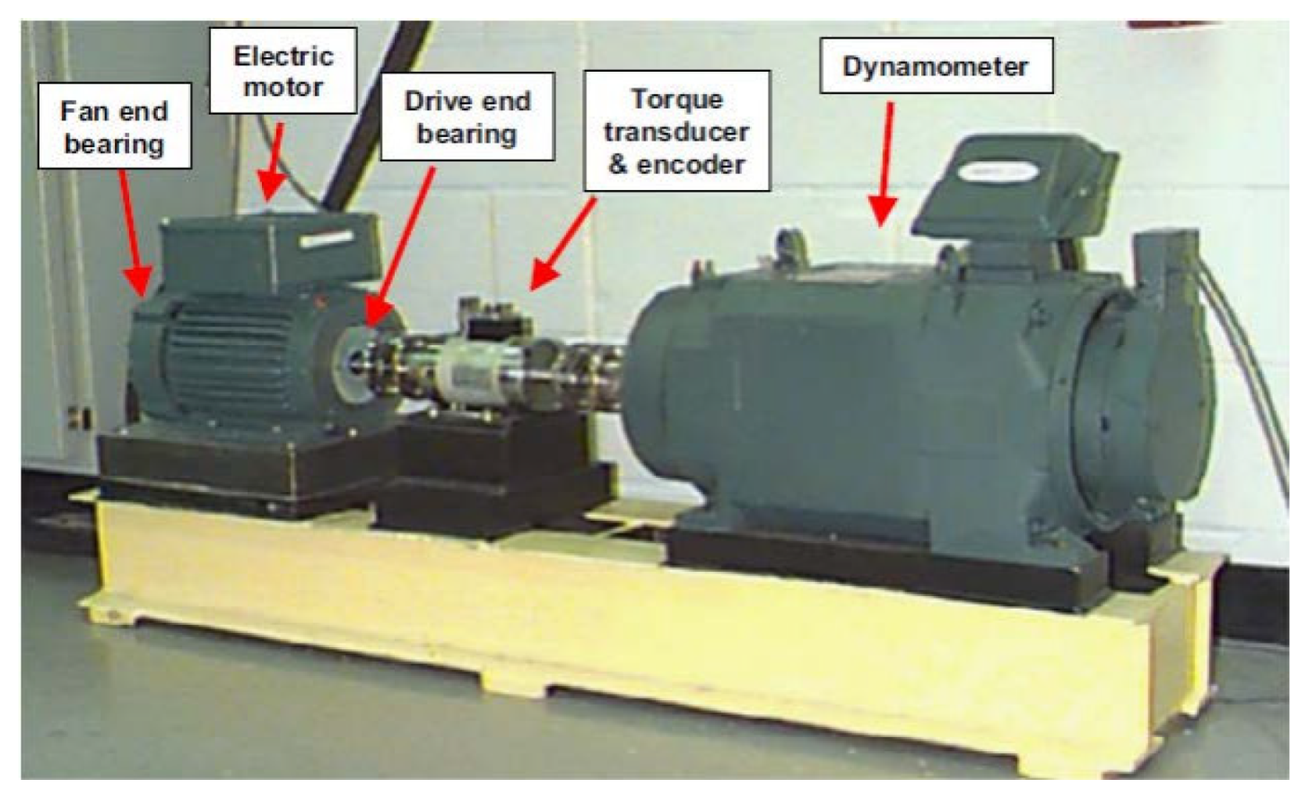
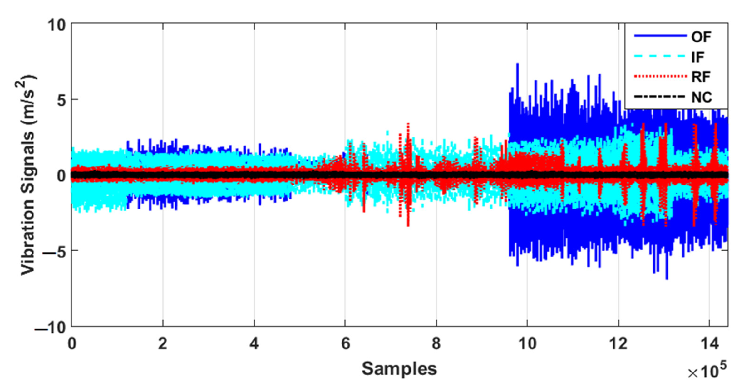
2. Dataset
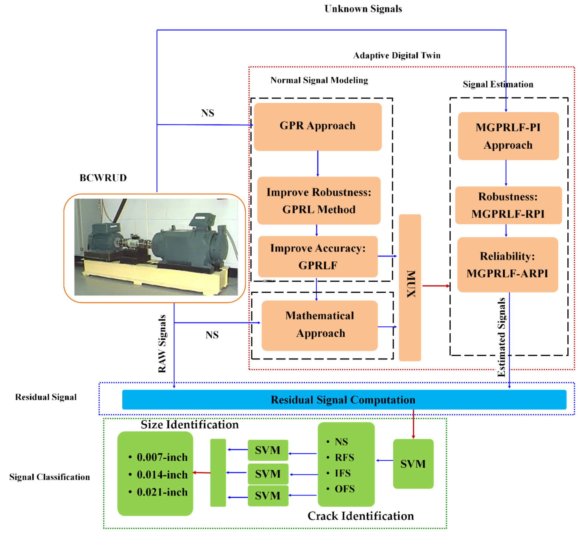
3. Proposed Scheme
3.1. Adaptive Digital Twin
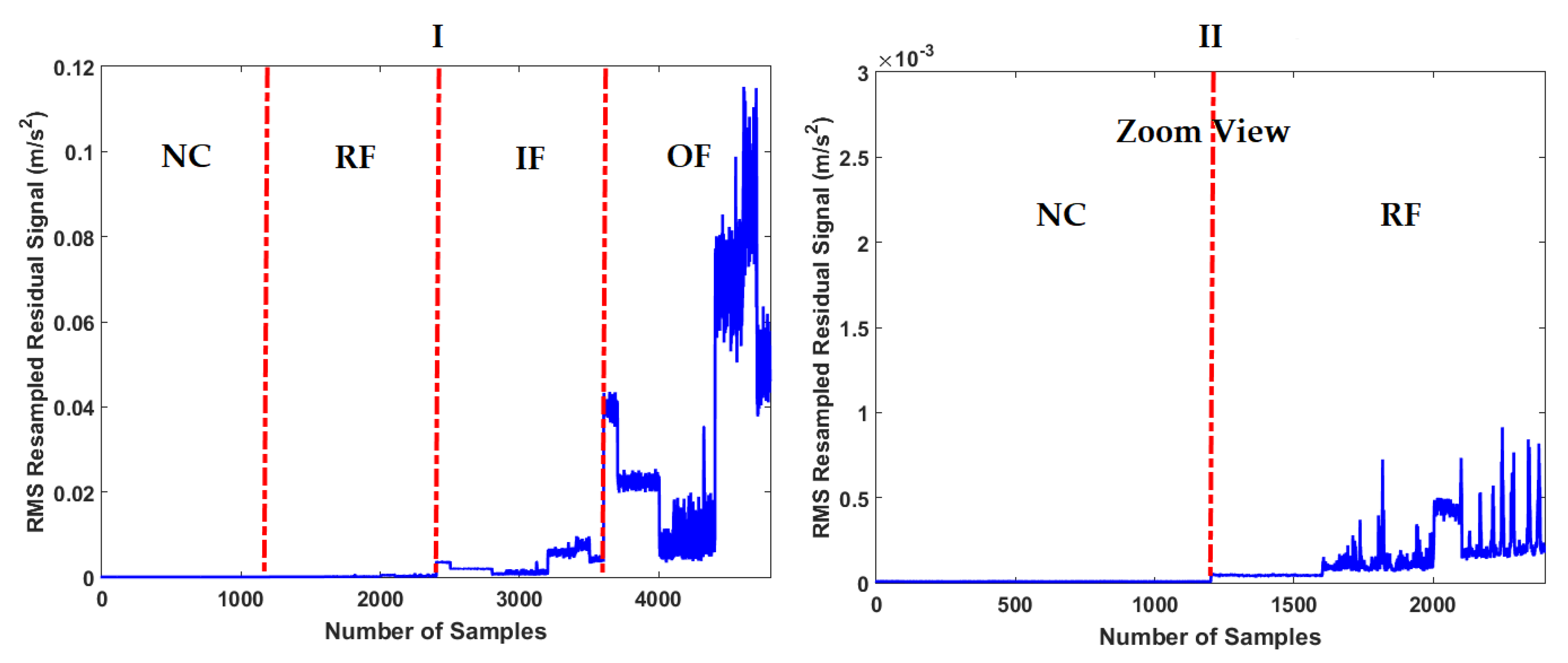
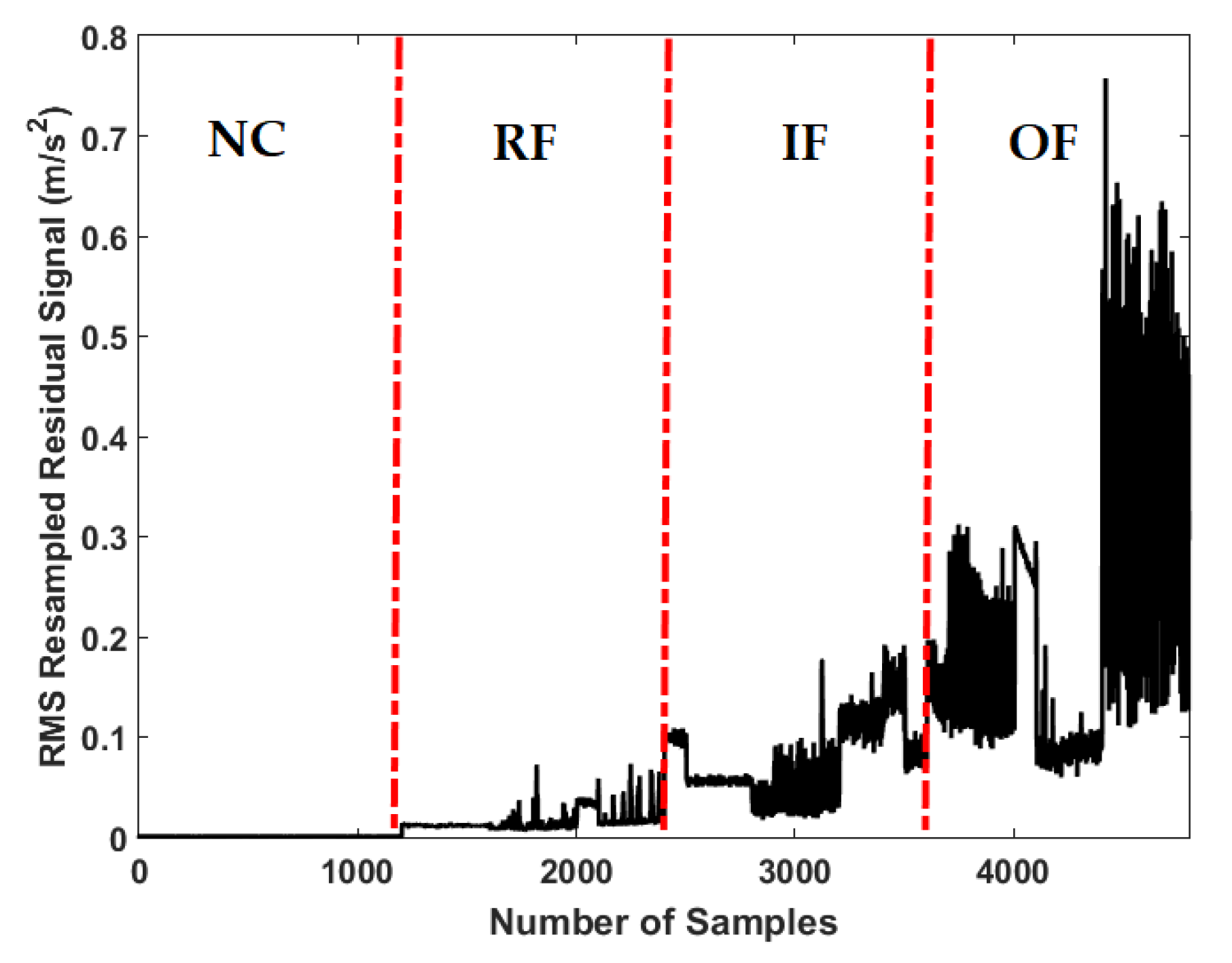
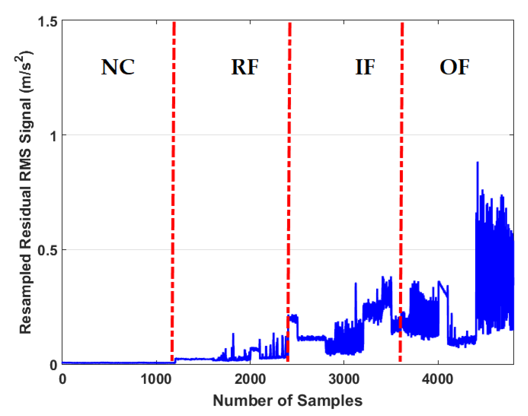
3.2. Residual Signal Computation
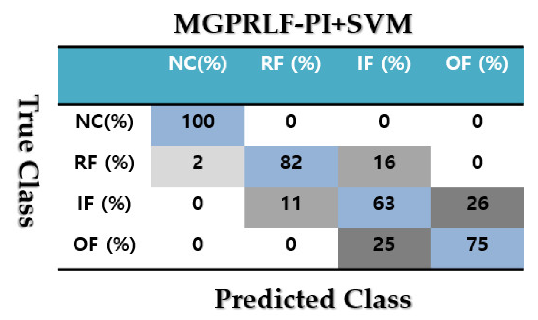
3.3. Signal Classification
4. Experimental Result
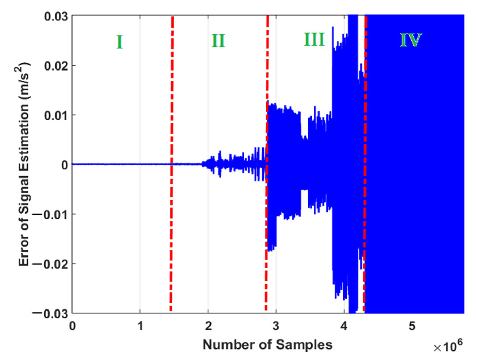
4.1. Signal Modeling and Estimation Using the ADT Results
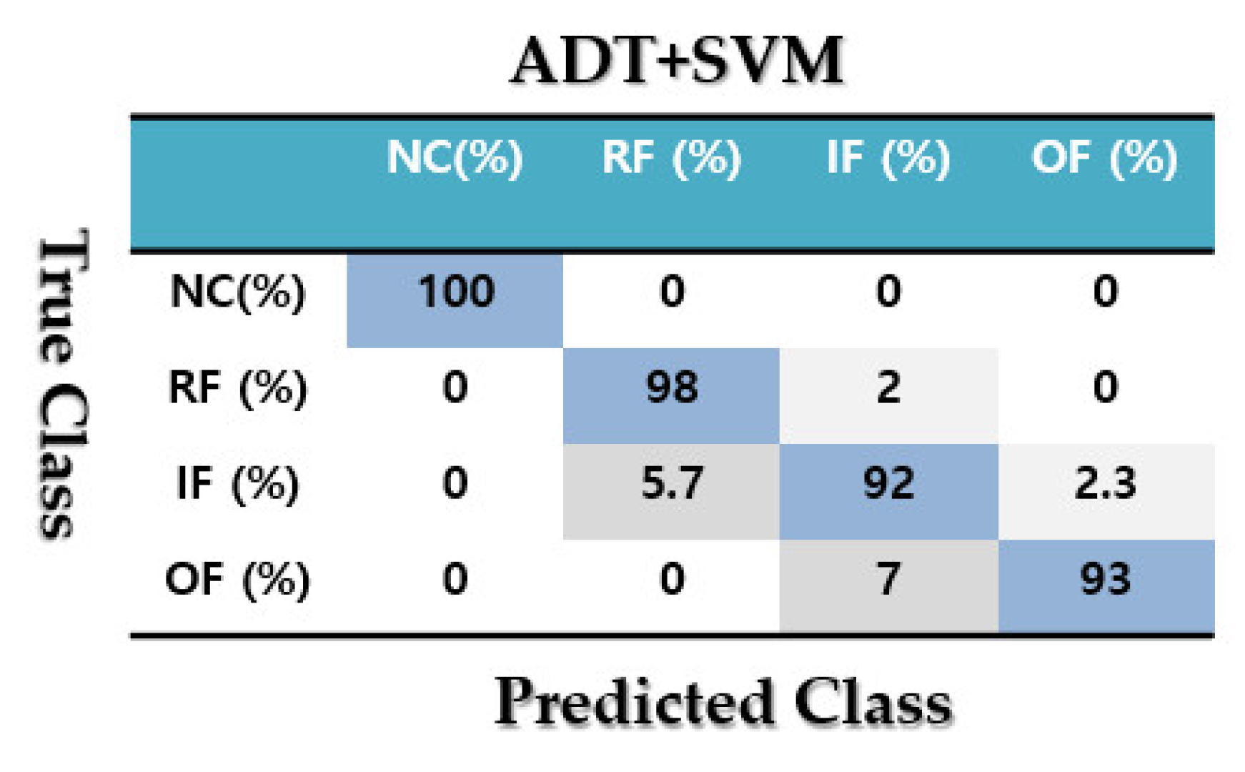
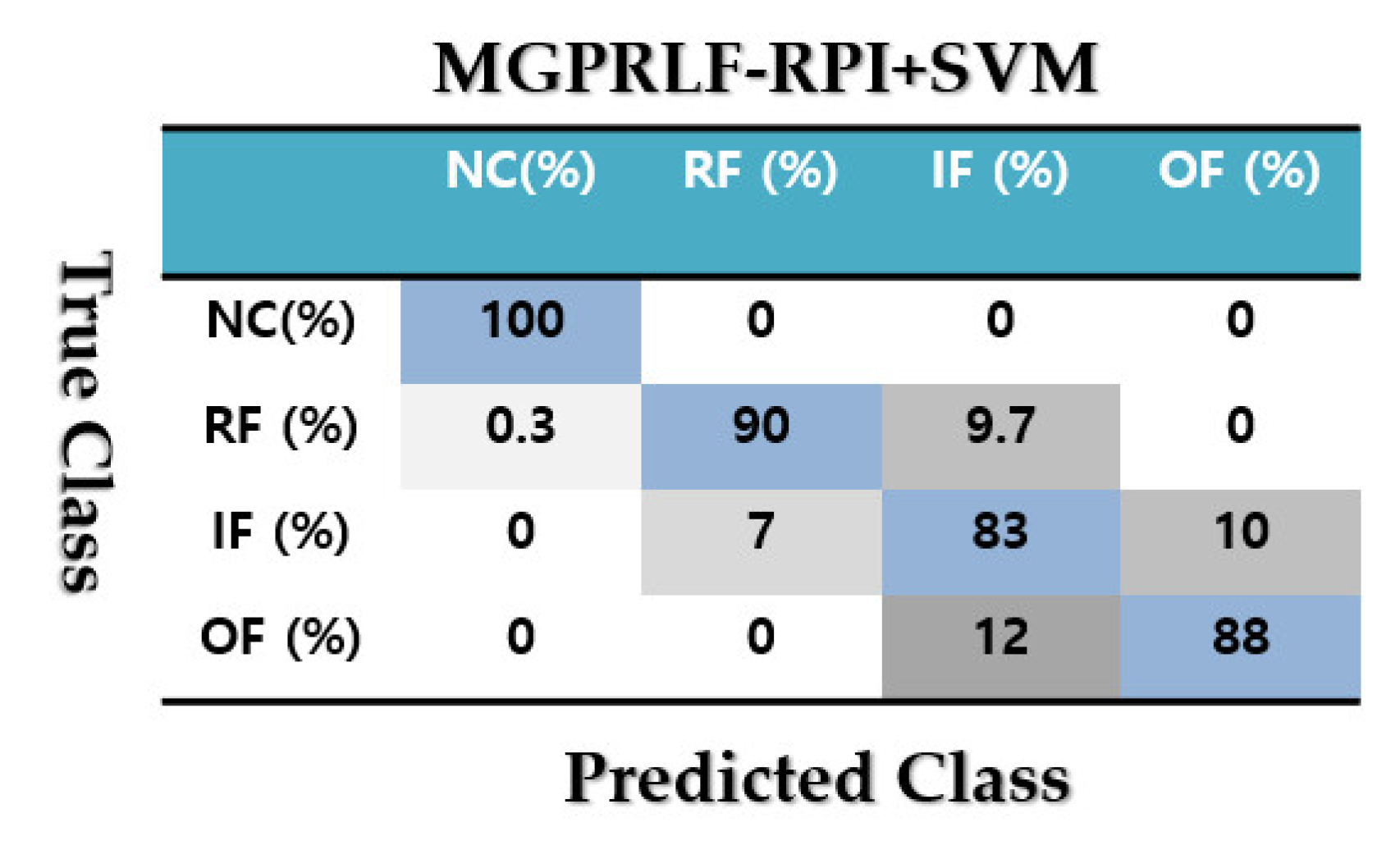
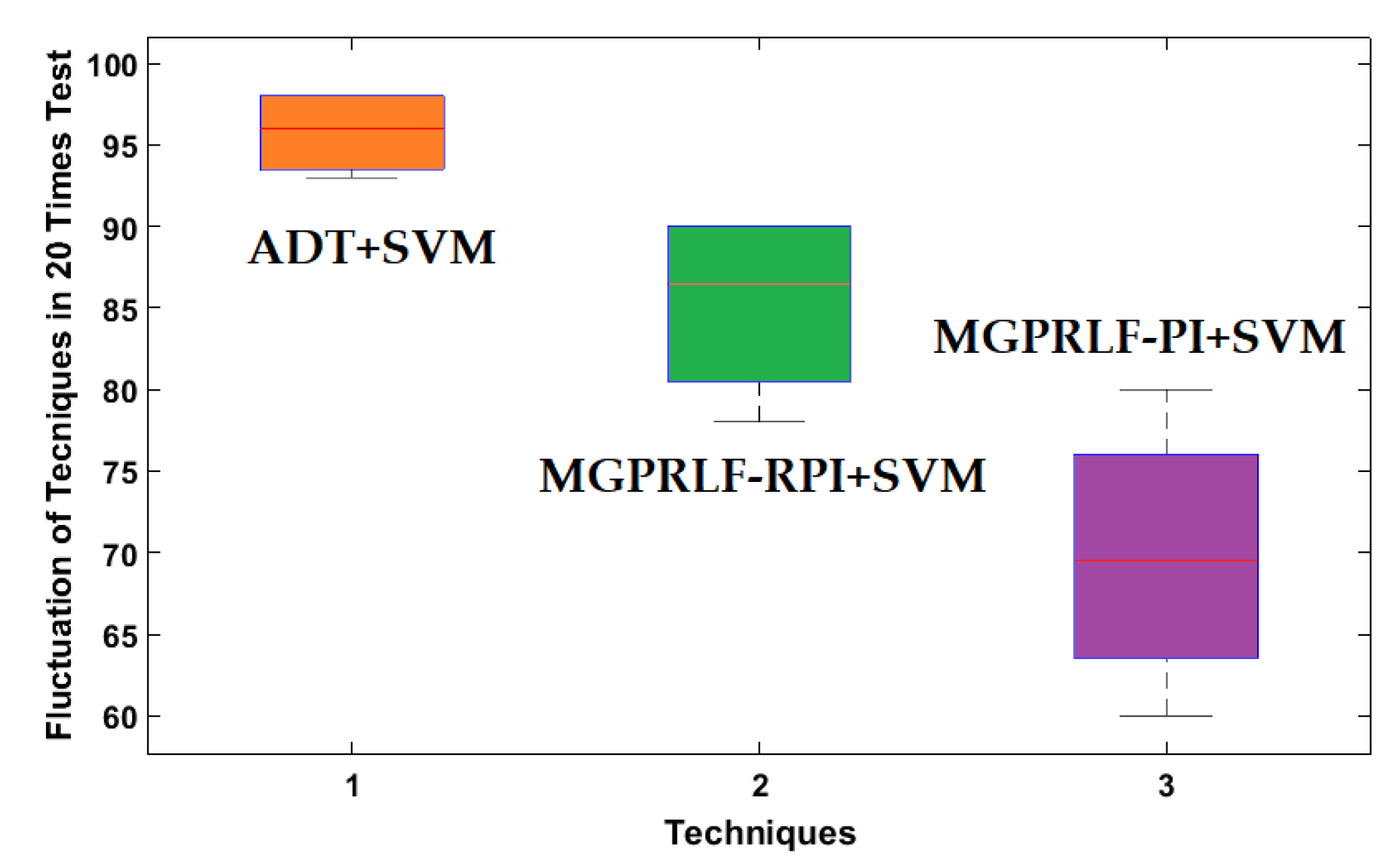
4.2. Fault Pattern Recognition (Crack Identification)
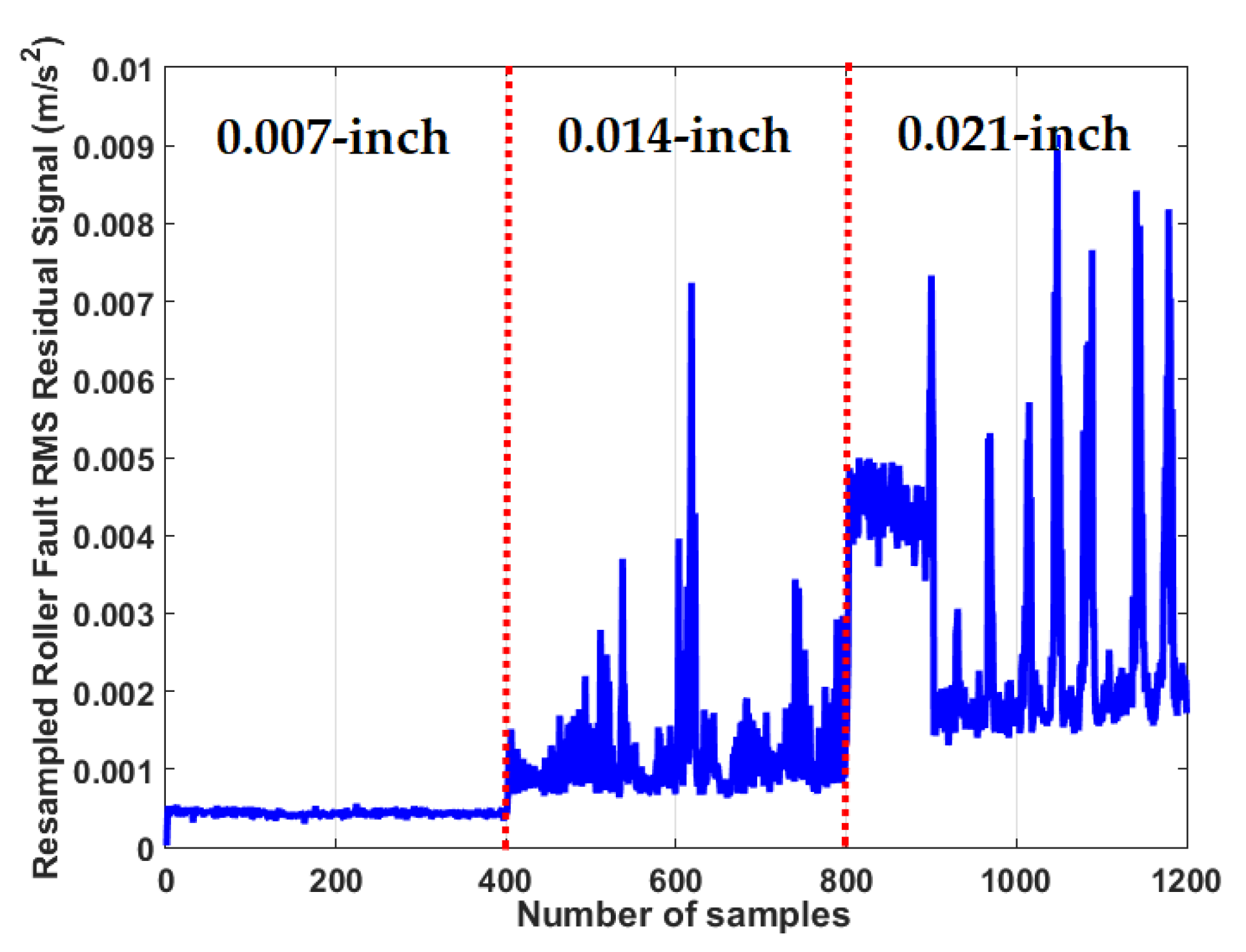
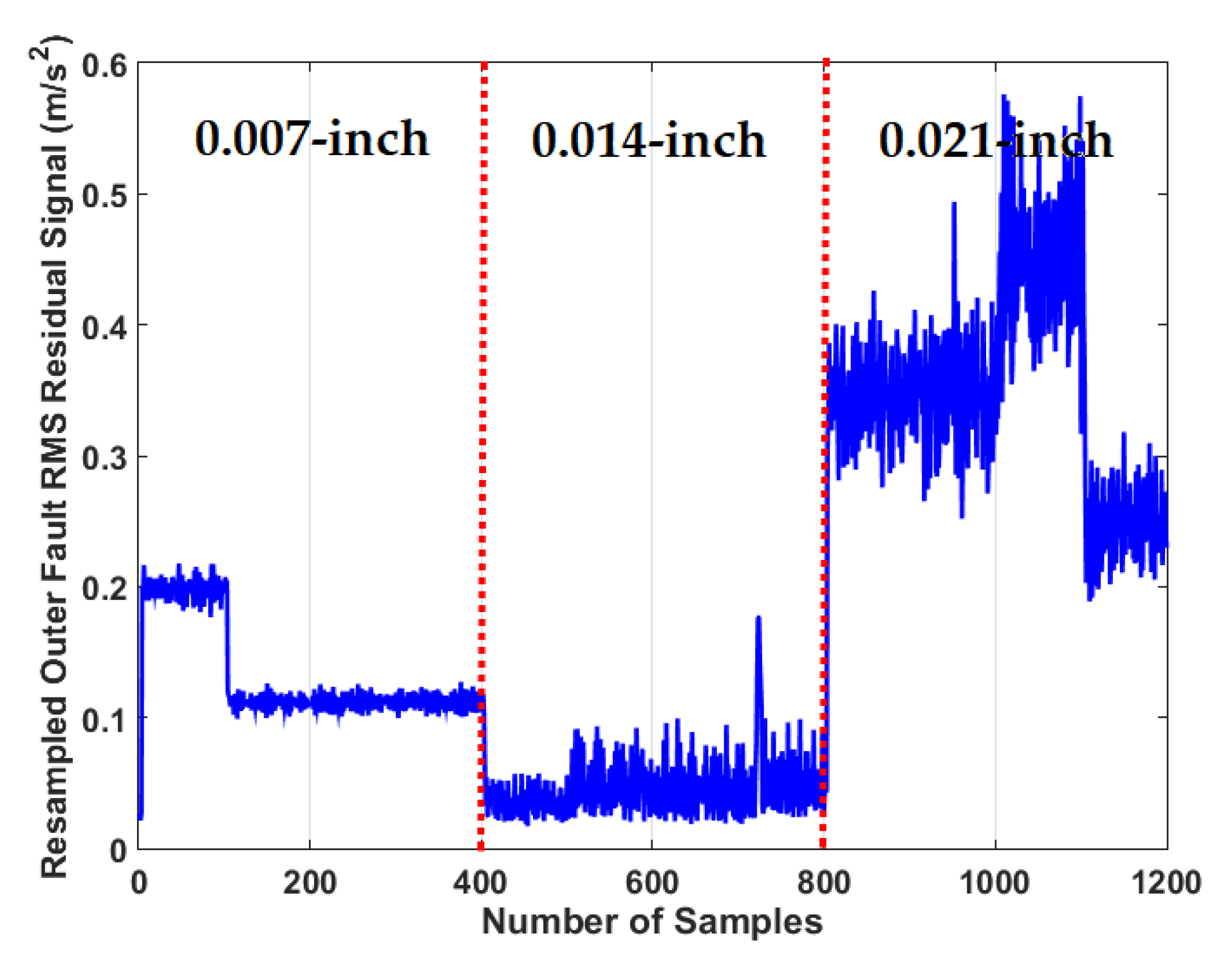
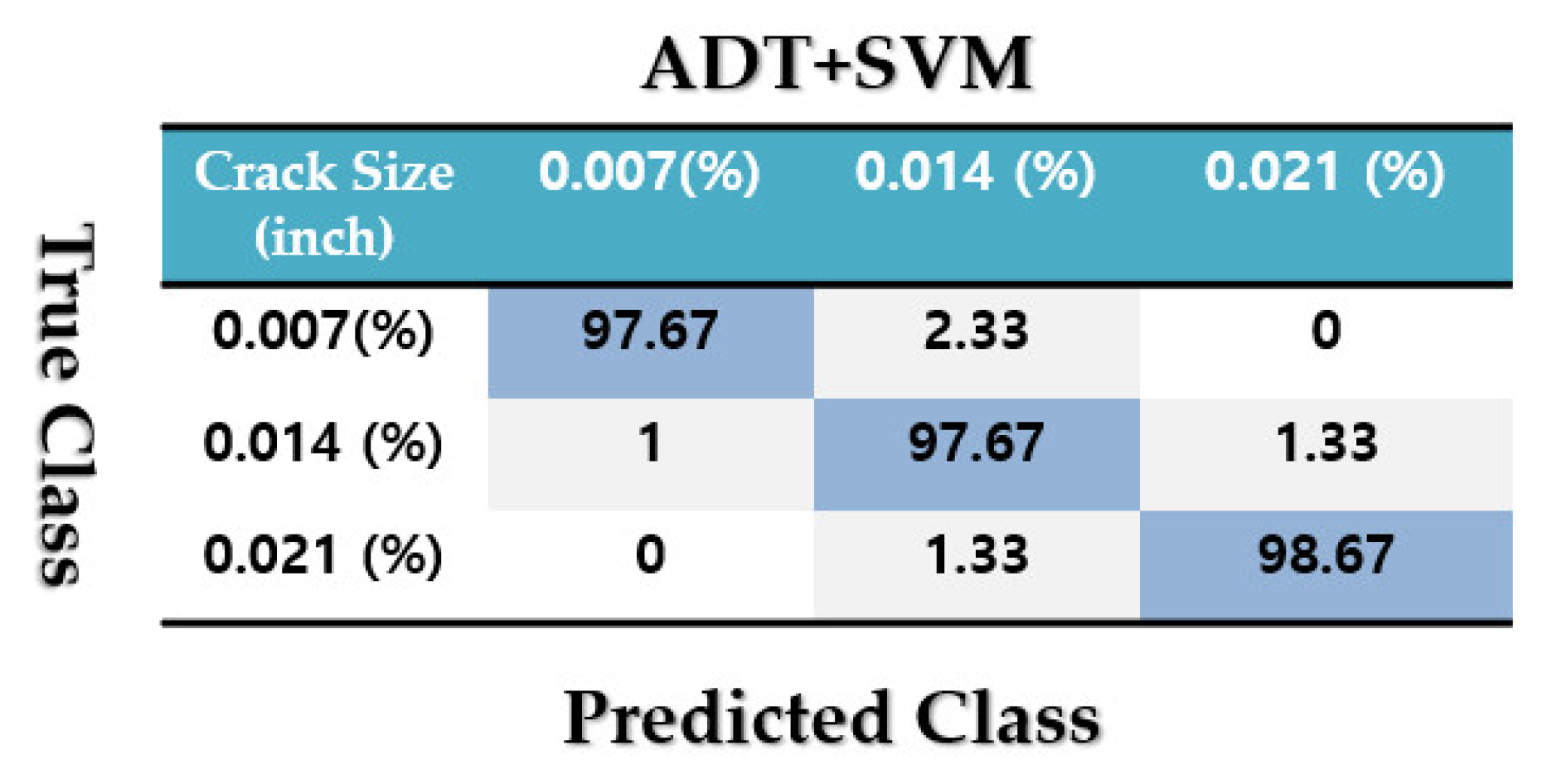
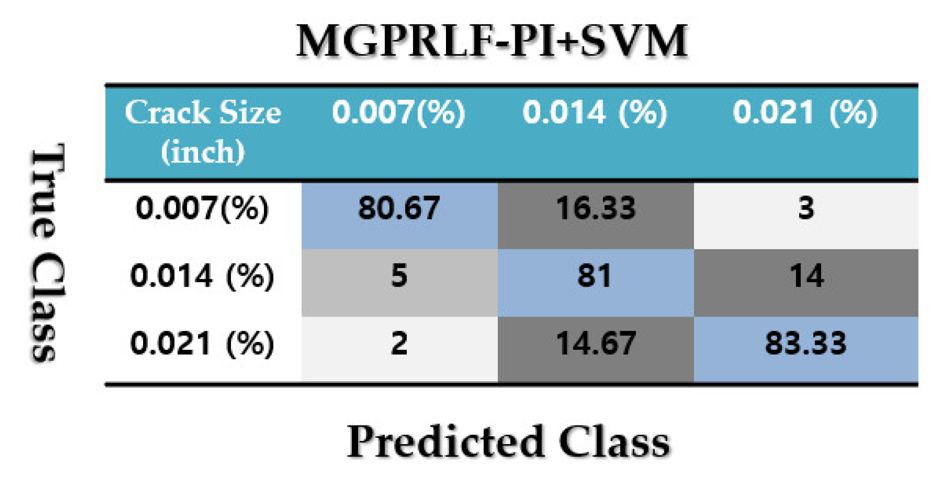
4.3. Crack Size Identification
5. Conclusions
Author Contributions
Funding
Data Availability Statement
Acknowledgments
Conflicts of Interest
Nomenclature
| ADT | Adaptive Digital Twin |
| SVM | Support Vector Machine |
| GPR | Gaussian Process Regression |
| PI | Proportional Integral |
| NC | Normal Condition |
| IF | Inner Fault |
| hp | horsepower |
| GPRLF | The combination of GPRL and fuzzy approach |
| MGPRLF-PI | PI observer with MGPRLF modeling |
| MGPRLF-ARPI (ADT) | The combination of MGPRLF-RPI observer and adaptive approach that is called adaptive digital twin |
| The measurable vibration signal | |
| The signal modeled by the GPR technique | |
| The coefficient of signal modeling using the GPR algorithm | |
| Signal variance | |
| Kernel width | |
| The modeled signal by the GPRL method | |
| CoG | Center of Gravity |
| The error of signal modeling using the GPRLF algorithm | |
| The modeled signal using the fuzzy algorithm to improve the accuracy and flexibility | |
| The coefficient of the modeled signal using the fuzzy algorithm | |
| The mass of bearing matrices | |
| A nonlinear term for modeling the bearing | |
| The effect of the roller fault | |
| The effect of the outer fault | |
| The number of rollers in the bearing | |
| The nonlinear term of the bearing using mathematically based vibration modeling | |
| The state of the vibration signal modeling using the mathematical approach | |
| The coefficient | |
| The modeled signal by the GPRLF method | |
| The state of the bearing signal estimation using the MGPRLF-PI technique | |
| The original raw signals that are collected by the vibration sensor | |
| The Lyapunov function | |
| Differentiable function of the uncertainty (unknown) condition | |
| The state of the bearing signal estimation using the MGPRLF-RPI technique | |
| The Lyapunov function to increase the robustness of the proposed algorithm | |
| The state of the bearing signal estimation using the proposed ADT technique | |
| The uncertainty estimation using the proposed ADT algorithm | |
| The adaptive (update) coefficient for tuning the proposed ADT estimator | |
| Residual signal using proposed ADT method | |
| ADT + SVM | The combination of ADT and SVM |
| MGPRLF-PI + SVM | The combination of MGPRLF-PI and SVM |
| RMS | Root Means Square |
| CWRUBD | Case Western Reserve University Bearing Dataset |
| FIE | Fuzzy Inference Engine |
| RPM | Rotation Per Minute |
| RF | Roller Fault |
| OF | Outer Fault |
| GPRL | The combination of GPR and Laguerre technique |
| MGPRLF | The combination of mathematical modeling and GPRLF |
| MGPRLF-RPI | The combination of MGPRLF-PI observer and Lyapunov approach |
| The state of the bearing signal modeling using the GPR technique | |
| The error of signal modeling using the GPR algorithm | |
| The covariance matrix using the GPR technique | |
| Noise variance | |
| The error of signal modeling using the GPRL algorithm | |
| State of the bearing signal modeling using the GPRL technique | |
| The covariance matrix using the GPRL algorithm | |
| The state of the bearing signal modeling using the GPRLF technique | |
| The modeled signal by the GPRLF method | |
| The covariance matrix using the GPRLF algorithm | |
| The external source forces | |
| The acceleration vibration signal that is measured by a vibration sensor | |
| And the unknown condition (hence is called uncertainty) | |
| The effect of the inner fault | |
| The angular velocity of rotor | |
| The difference between two reference angular positions | |
| The uncertainty term of the bearing using mathematically based vibration modeling | |
| The modeled vibration signal using the mathematical technique | |
| The state of the bearing signal modeling using the MGPRLF technique | |
| The estimated signal by the MGPRLF-PI method | |
| The uncertainty estimation using the MGPRLF-PI algorithm | |
| The coefficient of PI observer | |
| The Hamilton–Jacobi discrimination | |
| The estimated signal by the MGPRLF-RPI method | |
| The uncertainty estimation using the MGPRLF-RPI algorithm | |
| The coefficient of the RPI technique | |
| The estimated signal by the proposed ADT method | |
| The effect of the Lyapunov function to improve the robustness in the proposed ADT algorithm | |
| The RMS resampled residual signal using proposed ADT | |
| T | The number of windows |
| MGPRLF-RPI + SVM | The combination of MGPRLF-RPI and SVM |
References
- Peeters, C.; Antoni, J.; Helsen, J. Blind filters based on envelope spectrum sparsity indicators for bearing and gear vibration-based condition monitoring. Mech. Syst. Signal Process. 2020, 138, 106556. [Google Scholar] [CrossRef]
- Zhang, H.; Zhang, C.; Wang, C.; Xie, F. A survey of non-destructive techniques used for inspection of bearing steel balls. Measurement 2020, 159, 107773. [Google Scholar] [CrossRef]
- Alshorman, O.; Irfan, M.; Saad, N.; Zhen, D.; Haider, N.; Glowacz, A.; Alshorman, A. A Review of Artificial Intelligence Methods for Condition Monitoring and Fault Diagnosis of Rolling Element Bearings for Induction Motor. Shock. Vib. 2020, 2020, 1–20. [Google Scholar] [CrossRef]
- Xu, G.; Hou, D.; Qi, H.; Bo, L. High-speed train wheel set bearing fault diagnosis and prognostics: A new prognostic model based on extendable useful life. Mech. Syst. Signal Process. 2021, 146, 107050. [Google Scholar] [CrossRef]
- Balle, F.; Beck, T.; Eifler, D.; Fitschen, J.H.; Schuff, S.; Steidl, G. Strain analysis by a total generalized variation regularized optical flow model. Inverse Probl. Sci. Eng. 2019, 27, 540–564. [Google Scholar] [CrossRef] [Green Version]
- Hartmann, C.; Weiss, H.A.; Lechner, P.; Volk, W.; Neumayer, S.; Fitschen, J.H.; Steidl, G. Measurement of strain, strain rate and crack evolution in shear cutting. J. Mater. Process. Technol. 2021, 288, 116872. [Google Scholar] [CrossRef]
- Zhong, J.-H.; Wong, P.K.; Yang, Z.-X. Fault diagnosis of rotating machinery based on multiple probabilistic classifiers. Mech. Syst. Signal Process. 2018, 108, 99–114. [Google Scholar] [CrossRef]
- Xu, Y.; Li, Z.; Wang, S.; Li, W.; Sarkodie-Gyan, T.; Feng, S. A Hybrid Deep-Learning Model for Fault Diagnosis of Rolling Bearings. Measurement 2020, 169, 108502. [Google Scholar] [CrossRef]
- Song, L.; Wang, H.; Chen, P. Intelligent diagnosis method for machinery by sequential auto-reorganization of histogram. ISA Trans. 2019, 87, 154–162. [Google Scholar] [CrossRef]
- Piltan, F.; Kim, J.-M. Bearing Fault Diagnosis by a Robust Higher-Order Super-Twisting Sliding Mode Observer. Sensors 2018, 18, 1128. [Google Scholar] [CrossRef] [Green Version]
- Zmarzły, P. Multi-Dimensional Mathematical Wear Models of Vibration Generated by Rolling Ball Bearings Made of AISI 52100 Bearing Steel. Materials 2020, 13, 5440. [Google Scholar] [CrossRef] [PubMed]
- Piltan, F.; Kim, J.-M. Nonlinear Extended-state ARX-Laguerre PI Observer Fault Diagnosis of Bearings. Appl. Sci. 2019, 9, 888. [Google Scholar] [CrossRef] [Green Version]
- Li, X.; Yuan, C.; Li, X.; Wang, Z. State of health estimation for Li-Ion battery using incremental capacity analysis and Gaussian process regression. Energy 2020, 190, 116467. [Google Scholar] [CrossRef]
- Soualhi, A.; Medjaher, K.; Celrc, G.; Razik, H. Prediction of bearing failures by the analysis of the time series. Mech. Syst. Signal Process. 2020, 139, 106607. [Google Scholar] [CrossRef]
- Bai, Y.-T.; Wang, X.-Y.; Jin, X.-B.; Zhao, Z.-Y.; Zhang, B.-H. A Neuron-Based Kalman Filter with Nonlinear Autoregressive Model. Sensors 2020, 20, 299. [Google Scholar] [CrossRef] [Green Version]
- Khaleghi, S.; Karimi, D.; Beheshti, S.H.; Hosen, S.; Behi, H.; Berecibar, M.; van Mierlo, J. Online health diagnosis of lithium-ion batteries based on nonlinear autoregressive neural network. Appl. Energy 2021, 282, 116159. [Google Scholar] [CrossRef]
- Piltan, F.; Kim, J.-M. Bearing Fault Diagnosis Using an Extended Variable Structure Feedback Linearization Observer. Sensors 2018, 18, 4359. [Google Scholar] [CrossRef] [PubMed] [Green Version]
- TayebiHaghighi, S.; Koo, I. SVM-Based Bearing Anomaly Identification with Self-Tuning Network-Fuzzy Robust Proportional Multi Integral and Smart Autoregressive Model. Appl. Sci. 2021, 11, 2784. [Google Scholar] [CrossRef]
- Piltan, F.; Kim, J.-M. Advanced fuzzy-based leak detection and size estimation for pipelines. J. Intell. Fuzzy Syst. 2020, 38, 947–961. [Google Scholar] [CrossRef]
- Piltan, F.; Kim, J.-M. Fault Diagnosis of Bearings Using an Intelligence-Based Autoregressive Learning Lyapunov Algorithm. Int. J. Comput. Intell. Syst. 2021, 14, 537. [Google Scholar] [CrossRef]
- Mu, Y.; Zhang, H.; Xi, R.; Gao, Z. State and Fault Estimations for Discrete-Time T-S Fuzzy Systems with Sensor and Actuator Faults. IEEE Trans. Circuits Syst. II Express Briefs 2021, 1. [Google Scholar] [CrossRef]
- Sharafian, A.; Sharifi, A.; Zhang, W. Fractional sliding mode based on RBF neural network observer: Application to HIV infection mathematical model. Comput. Math. Appl. 2020, 79, 3179–3188. [Google Scholar] [CrossRef]
- Luo, W.; Hu, T.; Ye, Y.; Zhang, C.; Wei, Y. A hybrid predictive maintenance approach for CNC machine tool driven by Digital Twin. Robot. Comput. Manuf. 2020, 65, 101974. [Google Scholar] [CrossRef]
- Shervin, M.; Kalchbrenner, N.; Cambria, E.; Nikzad, N.; Chenaghlu, M.; Gao, J. Deep Learning-based Text Classification: A Comprehensive Review. ACM Comput. Surv. 2021, 54, 1–40. [Google Scholar]
- Li, J.P.; Haq, A.U.; Din, S.U.; Khan, J.; Khan, A.; Saboor, A. Heart Disease Identification Method Using Machine Learning Classification in E-Healthcare. IEEE Access 2020, 8, 107562–107582. [Google Scholar] [CrossRef]
- Wang, Z.; Yao, L.; Cai, Y. Rolling bearing fault diagnosis using generalized refined composite multiscale sample entropy and optimized support vector machine. Measurement 2020, 156, 107574. [Google Scholar] [CrossRef]
- Bearing Data Center. Case Western Reserve University Seeded Fault Test Data. Available online: https://csegroups.case.edu/bearingdatacenter/pages/welcome-case-western-reserve-university-bearing-data-center-website (accessed on 23 December 2020).
- Piltan, F.; Kim, J.-M. Bearing Anomaly Recognition Using an Intelligent Digital Twin Integrated with Machine Learning. Appl. Sci. 2021, 11, 4602. [Google Scholar] [CrossRef]
- Yueming, J.; Yu, Y.; Peng, X. Online Anomaly Detection in DC/DC Converters by Statistical Feature Esti-mation Using GPR and GA. IEEE Trans. Power Electron. 2020, 35, 10945–10957. [Google Scholar]
- Tanveer, M.; Ganaie, M.A.; Suganthan, P.N. Ensemble of classification models with weighted functional link net-work. Appl. Soft Comput. 2021, 107, 107322. [Google Scholar] [CrossRef]


| Information | Detail |
|---|---|
| Power of the induction motor | 2 [hp] |
| Bearing rotating speeds | 1730 [RPM]; 1750 [RPM]; 1772 [RPM]; 1797 [RPM] |
| Crack sizes | 0.007 [inches]; 0.014 [inches]; 0.021 [inch] |
| Sampling rate frequency | 48 [KHz] |
| Type of bearing | 6205-2RS JEM SKF |
| Number of rollers | 9 |
| Roller’s stiffness | |
| Outer’s stiffness | |
| Shaft’s stiffness | |
| Outer’s Mass | |
| Shaft’s Mass | |
| Defect depth | |
| Pitch diameter | |
| Roller diameter |
| Classes | Motor Torque Load [hp] | Crack Sizes [inch] |
|---|---|---|
| NC | 0,1,2,3 | - |
| RF | 0,1,2,3 | 0.007; 0.014; 0.021 |
| IF | 0,1,2,3 | 0.007; 0.014; 0.021 |
| OF | 0,1,2,3 | 0.007; 0.014; 0.021 |
| Conditions | Number of Training Samples | Number of Testing Samples |
|---|---|---|
| Crack Identification | ||
| NC | 900 | 300 |
| RF | 900 | 300 |
| IF | 900 | 300 |
| OF | 900 | 300 |
| Size Identification for RF | ||
| 0.007-inch | 300 | 100 |
| 0.014-inch | 300 | 100 |
| 0.021-inch | 300 | 100 |
| Size Identification for IF | ||
| 0.007-inch | 300 | 100 |
| 0.014-inch | 300 | 100 |
| 0.021-inch | 300 | 100 |
| Size Identification for OF | ||
| 0.007-inch | 300 | 100 |
| 0.014-inch | 300 | 100 |
| 0.021-inch | 300 | 100 |
| 1: | Adaptive Digital Twin Design Implement the state-space GPR algorithm, Equation (1). |
| 2: | Improve the robustness of autoregressive technique by combining autoregressive algorithm with the Laguerre filter. Equations (3) and (4) |
| 3: | Improve the accuracy and flexibility of GPRL using the GPRLF algorithm, Equation (9). |
| 4: | Mathematical modeling of the bearing, Equation (19). |
| 5: | Improve the performance of modeling in the digital twin using the MGPRLF algorithm, Equation (20). |
| 6: | Implement the combination of PI observer and MGPRLF for signal estimation, Equations (21) and (22). |
| 7: | Improve the robustness of MGPRLF-PI for signal estimation using MGPRLF-RPI, Equations (24) and (25). |
| 8: | signal estimation using the proposed ADT, Equations (26) and (27). |
| 9: | Residual Signal Computation Compute the residual signals, Equation (29). |
| Residual Signals Fault Classification | |
| 10: | Compute the resampled RMS residual signals, Equation (30). |
| 11: | Perform classification of the resampled RMS residual signals using the SVM [20,23]. |
| Classes | ADT +SVM (%) | MGPRLF-RPI +SVM (%) | MGPRLF-RPI +SVM (%) |
|---|---|---|---|
| NC | 100 | 100 | 100 |
| RF | 98 | 90 | 82 |
| IF | 92 | 83 | 63 |
| OF | 93 | 88 | 75 |
| Average | 95.75 | 90.25 | 80 |
| Size (inch) | ADT +SVM (%) | MGPRLF-RPI +SVM (%) | MGPRLF-RPI +SVM (%) |
|---|---|---|---|
| 0.007 | 98 | 90 | 80 |
| 0.014 | 96 | 88 | 82 |
| 0.021 | 98 | 89 | 80 |
| Average | 97.33 | 89 | 80.67 |
| Size (inch) | ADT +SVM (%) | MGPRLF-RPI +SVM (%) | MGPRLF-RPI +SVM (%) |
|---|---|---|---|
| 0.007 | 98 | 90 | 82 |
| 0.014 | 98 | 86 | 81 |
| 0.021 | 99 | 90 | 84 |
| Average | 98.33 | 88.67 | 82.33 |
| Size (inch) | ADT +SVM (%) | MGPRLF-RPI +SVM (%) | MGPRLF-RPI +SVM (%) |
|---|---|---|---|
| 0.007 | 97 | 91 | 80 |
| 0.014 | 99 | 88 | 80 |
| 0.021 | 99 | 88 | 86 |
| Average | 98.33 | 89 | 82 |
Publisher’s Note: MDPI stays neutral with regard to jurisdictional claims in published maps and institutional affiliations. |
© 2021 by the authors. Licensee MDPI, Basel, Switzerland. This article is an open access article distributed under the terms and conditions of the Creative Commons Attribution (CC BY) license (https://creativecommons.org/licenses/by/4.0/).
Share and Cite
Piltan, F.; Kim, J.-M. Crack Size Identification for Bearings Using an Adaptive Digital Twin. Sensors 2021, 21, 5009. https://doi.org/10.3390/s21155009
Piltan F, Kim J-M. Crack Size Identification for Bearings Using an Adaptive Digital Twin. Sensors. 2021; 21(15):5009. https://doi.org/10.3390/s21155009
Chicago/Turabian StylePiltan, Farzin, and Jong-Myon Kim. 2021. "Crack Size Identification for Bearings Using an Adaptive Digital Twin" Sensors 21, no. 15: 5009. https://doi.org/10.3390/s21155009
APA StylePiltan, F., & Kim, J.-M. (2021). Crack Size Identification for Bearings Using an Adaptive Digital Twin. Sensors, 21(15), 5009. https://doi.org/10.3390/s21155009