Estimation of Earthquake Early Warning Parameters for Eastern Gulf of Corinth and Western Attica Region (Greece). First Results

Abstract

The main goal of an Earthquake Early Warning System (EEWS) is to alert before the arrival of damaging waves using the first seismic arrival as a proxy, thus becoming an important operational tool for real-time seismic risk management on a short timescale. EEWSs are based on the use of scaling relations between parameters measured on the initial portion of the seismic signal after the arrival of the first wave. To explore the plausibility of EEWSs around the Eastern Gulf of Corinth and Western Attica, amplitude and frequency-based parameters, such as peak displacement (P_d), the integral of squared velocity ($I_{V }^2)$ and the characteristic period (τ_c), were analyzed. All parameters were estimated directly from the initial 3 s, 4 s, and 5 s signal windows (t_w) after the P arrival. While further study is required on the behavior of the proxy quantities, we propose that the $I_{V }^2$ parameter and the peak amplitudes of the first seconds of the P waves present significant stability and introduce the possibility of a future on-site EEWS for areas affected by earthquakes located in the Eastern Gulf of Corinth and Western Attica. Parameters related to regional-based EEWS need to be further evaluated.

1. Introduction

The increasing urbanization worldwide has led to the establishment of large metropolitan areas near major active faults (whether on land or offshore), which pose a serious threat to the human population and infrastructures. Currently, an accurate earthquake forecast method appears to be far from operational. Consequently, attention has shifted to Earthquake Early Warning Systems (EEWS) for reducing earthquake risk [1,2,3,4,5,6], offering, in real-time, information for the incoming destructive seismic waves. EEWS leverage the nature of the different seismic waves; since “P waves carry information while S waves carry energy” [7], the fast, yet low amplitude P waves are analyzed to determine the earthquake damage potential, mostly caused by the slower, high-amplitude S-waves.

Over the last two decades, due to rapid technological advances in the fields of signal processing and data transmission, effective techniques have been developed to analyze seismological data in almost real-time [7,8,9,10]. In this direction, real-time seismology integrates fast and instantaneous data broadcast systems with automatic signal processing, providing reliable estimates of earthquake parameters (location and magnitude) in the first few seconds during its occurrence [10]. Modern EEWSs can offer a few to tens of seconds of warning time for impending ground motions, allowing for mitigation measures in the short term [11,12]—such an approach is in use in Japan [2], Taiwan [13,14], Mexico [11], and the United States of America [15]. The information produced by the aforementioned systems can be used by civil protection authorities to minimize the damages and losses (human and economic) [16,17].

In most EEWSs, the peak amplitudes of displacement (P_d), along with the integral of squared velocity ($I_{V }^2$) parameter estimated from the initial Pwave, scales with the earthquake magnitude and peak ground acceleration (PGA) [17,18,19]. This suggests that we can predict the earthquake magnitude and the intensity of the ground motion using the initial P waves. It is still under scientific debate whether determining the attenuation relationship of P_d naturally leads to practical applications for early warning. We note that recently the time evolution of P_d was investigated, suggesting a universal pattern of initial growth that is inconsistent with deterministic models of earthquake rupture [19]. Therefore, when a large earthquake occurs, its location can be quickly obtained from a few P wave arrival times at nearby stations, and P_d can then be used to determine its magnitude via the attenuation relationship, which can then be used in the EEWS for emergency operations.

Earthquake early warning systems can mainly be divided into two categories: (a) on-site and (b) regional. The on-site EEWS use one seismic station, while the regional approach requires a seismic network [20]. This poses fundamental differences in the design, operation, and maintenance of the EEWS. In (b), the time between the event origin and the alert emission is reduced, as it requires P wave triggers in multiple stations. By contrast, in (a), a single arrival is adequate. The above has obvious implications on the robustness of the emitted alert and whether it is false or not. On the other hand, on-site approaches avoid pitfalls in the earthquake and magnitude estimation (which, in turn, do not affect the quality of the alert). The development and implementation of regional EEWSs were summarized in a number of previous studies [6,20], along with some very recent approaches that predict seismic intensity at a target site based on the seismic intensities observed at seismic stations around the target site [21]. This type of EEWS requires the arduous task of designing and deploying a network of sensors with specific geometry and specifications (as opposed to on-site systems that require either a single or a few instruments). In general, the discussion about EEWSs’ limitations is ongoing, with questions, such as the physical boundaries of warning times in relation to the level of ground motion, exist and are still open [22,23].

In this work, we analyze parameters that are used to determine earthquake magnitude in real-time for the areas of the Eastern Gulf of Corinth (EGoC) and Western Attica (WA). We focused on the correlation of (a) P_d (as both a regional and an on-site proxy) with the magnitude M_w and the hypocentral distance H, (b) the characteristic period τ_c with magnitude, averaged over the area, (c) the integral of squared velocity ($I_{V }^2$) with PGA on-site and inter-site. The latter aims to investigate whether it is possible to use P waves near the source as a proxy for S-wave shaking at a far target. In that context, we also design relations between P_d,v,a and PGA, for inter-site use. Evaluating the practicability of an EEWS in this area is justified by its high level of seismic hazard. The area spans two zones of the New Greek Seismic Code (NEAK) with expected PGA values at a minimum of~157 cm/s² and a maximum of~353 cm/s² for a return period of 475 years (see Figure 1 in [24]). It is noted that the NEAK features four broadly defined zones with wide PGA ranges. Ref. [24] using a more refined model and various empirical Ground Motion Prediction Equations found expected PGA between 100 cm/s² and 300 cm/s². The European Seismic Hazard Map (ESHM13) by [25] confirms this by categorizing the area as high-hazard with an expected PGA of ~300 cm/s². Moreover, large oil refineries and power plants are located in the EGoC and the coast of WA. For them, suitable safety measures, such as automatic blocking of pipelines or gas lines to prevent fire hazards or the automatic shutdown of manufacturing operations to avoid valuable equipment exposure, could be adopted for damage reduction. Therefore, the introduction of an EEWS is a worthwhile objective because it can be effectively used to reduce the damage caused by the strongest earthquakes. It is noted that the effectiveness of an EEWS is multifaceted, with issues such as civil protection response [26] and network limitations factored in. In a recent feasibility study by [27], it was shown that events in the Eastern Gulf of Corinth could have a warning time of 10 s in Athens. We note that the Virtual Seismologist (VS) EEW software and PRESTo have been installed in the area of the Western Gulf of Corinth and Central Greece, and their initial performance has been presented [28,29].

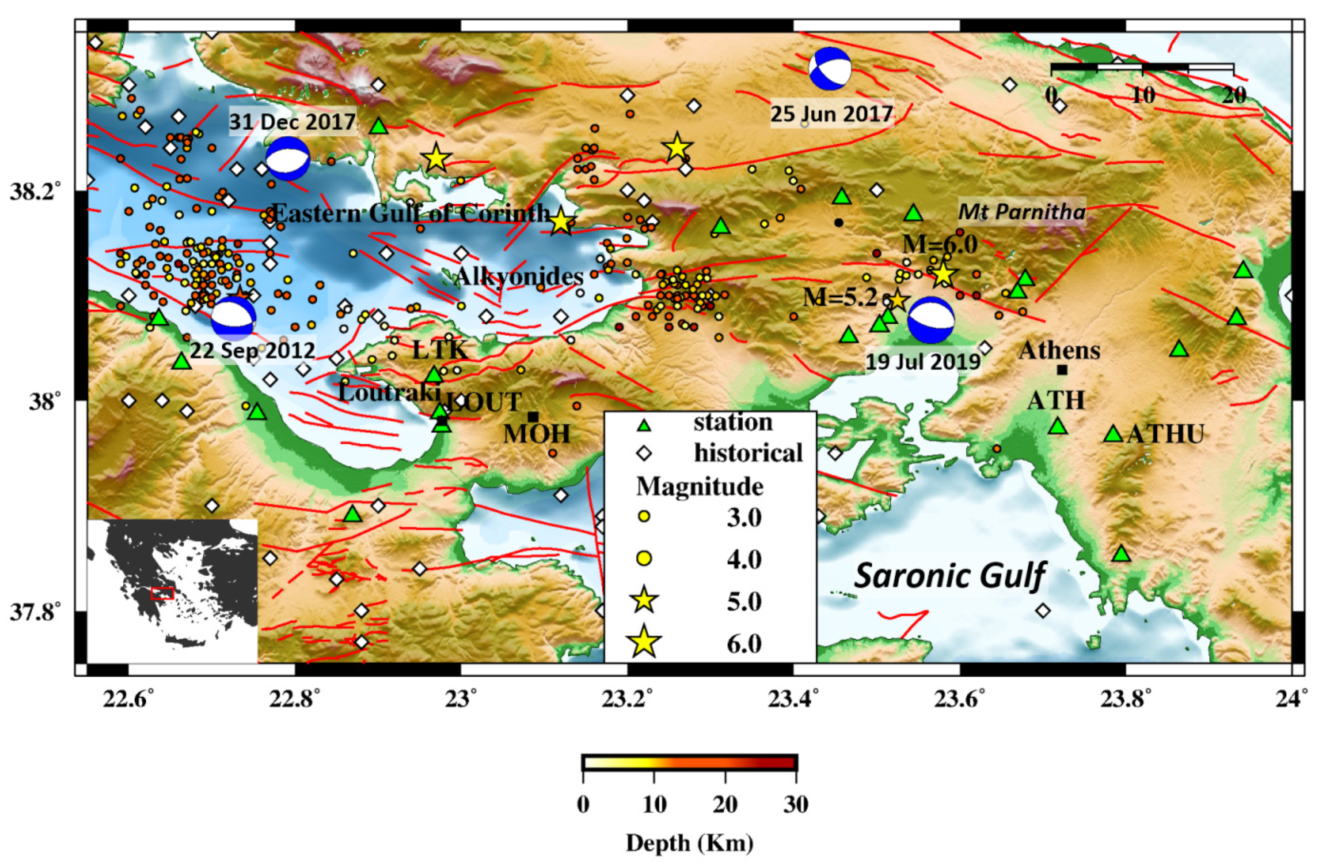
2. Seismotectonic Setting, Data Acquisition, and Processing

The Gulf of Corinth (GoC) is an important E–W oriented neotectonic half-graben, bounded by normal faults, gradually evolving during the Pleistocene, as it is evidenced by the intense seismic activity [30]. Normal faults continue from the Eastern end of the GoC (EGoC) towards the Saronic Gulf [31].

There are two main sources of strong earthquakes in the area: (a) the Parnitha range in WA and (b) the Alkyonides Islands in the EGoC. Parnitha acts as a NW boundary to the Athens basin. Its, generally, E–W and NE–SW trending faults are extended southward and have been the cause of earthquakes that have had a detrimental impact to Athens and the surrounding area. On 7 September 1999, a M_w = 6.0 event occurred at the southern part of Parnitha, about 20 km NW of Athens. The ferocity of the shaking led to billions of dollars in damage, decimated infrastructure, as well as hundreds of casualties [32]. Its shallow focus and proximity to the capital [33,34], as well as issues with constructions on unsuitable sites [35], were the culprits for the high intensities observed. More recently, in 2019, a M_w = 5.2 earthquake occurred in the same structure [36], acting as a reminder of the danger posed by active faults in the vicinity of Athens (Figure 1); other than a partial collapse of an abandoned building, the city was left unscathed, even though its western outskirts sustained some damage [37]. The region NW of Parnithta also hosts faults that cause shallow seismicity (with potential moderate to strong events) and, consequently, could have an impact on Athens [38]. Another source lies closer, NE of Athens, but has, so far, witnessed some felt events, such as the M_w = 4.2 earthquake of 2018 [39], without any noticeable impact on hazard, due to the weak magnitudes.

In Figure 1, a geotectonic map of the broader area of the Eastern Corinth Gulf and Western Attica is presented where all the events between 1900 and 2008 [40] along with the historical earthquake locations [41] and the faults are presented.

The islands of Alkyonides were the sole focus of seismic hazards associated with Athens and the Eastern Gulf of Corinth until 1999. A series of strong events between February and March of 1981, with magnitudes of M_w > 6.0 for three of them, caused unprecedented damages in the area [42]. Further study of the 1981 area implied the occurrence of several other similar events (in terms of deformation) in historical times, indicating the region as a prime contributor to regional seismic hazard [41,43]. Since then, the absence of strong events or significant seismicity led to a sparse seismological network, despite the region’s importance. Either Parnitha or Alkyonides could produce an earthquake that affects an area that includes a major city (Athens), a significant tourist hub (Loutraki), and industrial infrastructure, such as the oil refineries of the Motor Oil Hellas (MOH) group (Figure 1).

To estimate the scaling parameters for an EEWS in the area, we retrieved an event catalog for the Eastern Gulf of Corinth and Western Attica from the International Seismological Center (ISC), consisting of 278 earthquakes between January 2008 and February 2021, with a minimum magnitude of 3.0 and a maximum depth of 30.0 km. The catalog was obtained through ISC’s European Integrated Data Archive (EIDA) node, using the respective international Federation of Digital Seismograph Networks (FDSN) service. To homogenize the magnitudes, we used the relations proposed by [43,44] for converting to M_w. Then, we searched for waveform data in the archive of the Geodynamic Institute of the National Observatory of Athens (GI-NOA) through their EIDA node.Their database includes recordings provided by several Greek institutes, recorded by stations of the Hellenic Unified Seismological Network (HUSN) [45], and initially selected 33 suitable stations, including 24 velocimeters and 9 accelerometers. The GI-NOA node also includes detailed station metadata, such as the response functions of both velocimeters and accelerometers [46]. We set a maximum event search radius of 100.0 km around each station of interest. This set included two sites in Loutraki (LOUT and LTK) and two in Athens (ATH and ATHU). These sites feature long-term installations (ensuring a wealth of available data) and are located close to the two most important seismic sources around the local industrial infrastructure (e.g., oil refineries) and the metropolitan city of Athens, i.e., Alkyonides [41,42] and Parnitha [32,33,34,35,36,37]. All four stations have broadband sensors.

Data acquisition and signal processing (including instrument response removal and transformations between different ground motion outputs) was carried out using routines by ObsPy (see https://docs.obspy.org, accessed on 26 July 2021) [47]. To process the data, we first ensured that no clipped recordings were included by visually inspecting suspicious event-station pairs (i.e., seismographs located within 30.0 km of earthquakes with a magnitude of at least 4.5). Then, we automatically picked the arrival of the P-phase with the algorithm proposed by [48]. To estimate any EEWS parameter, we used three time-windows starting from the P arrival and extending to 3 s, 4 s, or 5 s (t_w). Since, in most cases, the used t_w is significantly larger than the expected automatic phase picking uncertainty, the results are expected to be largely unaffected by it. To remove noise that could lead to issues with the picker, we first applied a bandpass filter between 1.0 and 20.0 Hz. This filter was used exclusively in the picking process. Moreover, we estimated the S-P time with TauP [49] using a local velocity model [50]. The raw, unfiltered data were then deconvoluted with the instrument’s response to obtain the actual ground motions (i.e., displacement, velocity, and acceleration) at each site. After applying a high pass filter with a corner frequency of 0.075 Hz [51], we determined the peak value for each motion type (hereafter noted as P_d,u,a for displacement, velocity, and acceleration, respectively) in the three t_w, as well as the peak ground acceleration of the shear-waves (hereafter, called PGA) in a window ending 20 s after the theoretically estimated S arrival. However, if the signal window t_w exceeded the estimated S-P time, the measurement was rejected. We set the S-P time exceedance criterion to a priori avoid cases of overlapping windows for measurements of P peak and S peak amplitudes, as in the case of the t_w = 5 s window in Figure 2. The process was repeated for all available recordings and all three channels (Figure 2).

In the final dataset, we removed observations with a PGA to P_a ratio less than 2.0. This criterion was important to avoid cases of erroneous picking, inherent instrumentation issues (e.g., clock drifts), and problems with the instrument correction (e.g., errors or omissions in the provided instrument response for each epoch). The final dataset contains 2308 measurements among the three time-windows, for 240 events and 23 stations (947 event-station pairs).

Our observations span a magnitude range between 3.0 and 5.2 (Figure 3). There is a good distribution for lesser magnitudes; however, magnitudes above 4.5 present sporadic measurements, with large gaps, as in the case of the sole M_w = 5.2 event. Acceptable observations span a distance between ~20 km and ~50 km (Figure 3a). The signal-to-noise ratio (SNR, in dB), indicated an increase with magnitude (Figure 3b). However, we noted that the considered earthquakes were recorded in a variety of stations with different conditions. For example, two of the closest seismological stations to the M_w = 5.2 event were located in the city of Athens, largely affected by urban noise, which, as logic dictates, is a detriment to SNR.

3. Empirical Correlation Laws for Eastern Gulf of Corinth and Western Attica Region

Determinations of magnitude and the ground shaking intensity from the initial P wave are two important elements for earthquake early warning. The strength of shaking can practically be represented by PGA. Here we present the first results from an effort to establish the correlation laws required for regional EEWS (in Section 3.1 and Section 3.2) and that for on-site (in Section 3.3). We also explore the possibility of inter-site relations (in Section 3.4).

3.1. Peak Ground Displacement, Magnitude, and Distance

In [2,52], based on the P_d measured on the 3 s window starting from the P wave arrival, estimated the magnitude of a seismic event. Furthermore in [53,54] showed that P_d scales with the earthquake magnitude and could be used for its real-time estimation in EEWS applications. Using the P_d values estimated (in cm), we assume a simple linear regression model among the logarithm of P_d, the magnitude M and the logarithm of the hypocentral distance H (in km) as:

$$\log \left(P_d\right)=a+b\ast M+c\ast \log \left(H\right)$$

(1)

where a, b, and c are constants to be determined from the linear least-squares regression analysis. The resulting best fitting relationship for the two stations in Athens is presented in Figure 4 for the three signal windows.

For stations located in Athens (i.e., ATH and ATHU) and for the different t_w used, the mean relationships are:

$$\begin{array}{c}\log \left(P_d\right)=-3.846+0.605\ast M-1.474\ast \log \left(H\right),{ \mathrm{for} \mathrm{t}}_{\mathrm{w}}=3\mathrm{s} \\ \log \left(P_d\right)=-3.465+0.606\ast M-1.659\ast \log \left(H\right),{ \mathrm{for} \mathrm{t}}_{\mathrm{w}}=4\mathrm{s}\\ \log \left(P_d\right)=-2.972+0.627\ast M-1.927\ast \log \left(H\right),{ \mathrm{for} \mathrm{t}}_{\mathrm{w}}=5\mathrm{s}\end{array}$$

(2)

Standard deviations of intercepts for P_d relations in Athens ranged between 0.438 and 0.701. The magnitude’s factor deviation was between 0.067 and 0.096, while hypocentral-related constants were bounded by deviations within 0.205 and 0.364 (Figure 4). It is apparent that wider P wave windows yielded larger deviations. However, this cannot be considered as the sole metric of regression quality; thus, we also included the relevant correlation coefficients (Figure 4).

The regression constants are very close to the ones presented in [49] for Southern California. Regression results for the rest of the combinations between station and time windows are provided in the Supplementary Materials. We include 42 station-time window pairs with the corresponding regressions. The individual correlation coefficient and the number of observations used in the regression are also included.

Performing a regression over the whole dataset yields the relations shown in Figure 5. Lower magnitudes seem to correspond to more scattered values of P_d. Correcting the displacement by a factor determined by the hypocentral distance, as in [55,56], the relation $\log \left(P_d\right)-c\ast \log \left(H\right)=a+b\ast M$, exarcebates this issue (Figure 4b). Regressing for the two independent values (i.e., magnitude and distance) yielded a relatively higher correlation than the normalized ground amplitude approach (see Figure 4).

An alternative approach to correct the displacement by a factor determined by the hypocentral distance and a reference distance (in our case, H_ref = 100 km) is presented in [55], where $\log \left(P_d\frac{H}{H_{ref}}\right)=\alpha {\rm M}-b$, with α ≈ 0.84 and b ≈ 7.5, close to that presented in [56] for a regional EEWS application in Israel (Figure 5c), yielding a relatively higher correlation than the normalized ground amplitude approach (see Figure 4 and Figure 5).

To evaluate the predicted magnitude M_pred using Equation (2), we plotted it along with that observed M_obs (Figure 6). In this plot, the dichotomous line is presented. We observe that for all used three time-windows starting from the P arrival (i.e., t_w 3 s, 4 s, and 5 s), the majority of M_pred values were within ±0.5 units from that observed. Furthermore, the distribution of the ratio M_pred/M_obs and the deviation M_pred-M_obs are presented in the Appendix A.

Table 1. The average values of ration M_pred/M_obs and the deviation M_pred-M_obs for the t_w used.

tw	Mpred/Mobs	Mpred-Mobs
3 s	1.017 ± 0.18	0.05 ± 0.61
4 s	1.012 ± 0.17	0.034 ± 0.59
5 s	1.022 ± 0.19	0.07 ± 0.65

summarizes the average values indicate that the ration M_pred/M_obs is close to one while the deviation M_pred-M_obs close to zero for the t_w used.

3.2. The Characteristic Period τ_c

In Ref. [7] developed a different parameter called characteristic period (τ_c), which is an expression of the ratio between velocity and displacement records. This parameter is determined as follows: first, we compute $r=\frac{{{\displaystyle \int }}_{t_p}^{t_p+t_w}{\dot{u}}^2\left(t\right)dt}{{{\displaystyle \int }}_{t_p}^{t_p+t_w}{u}^2\left(t\right)dt}$ where u(t) is the ground motion displacement and $\dot{u}\left(t\right)$ the velocity. The integration is taken in the time window t_w after the arrival time t_p of P waves, then ${\tau }_c=\frac{2\pi }{\sqrt{r}}$ in s. Data from both velocity and acceleration recorders have been used to estimate τ_c in several seismic regions, demonstrating that the characteristic period scales with seismic event magnitude [6,57,58,59,60]. Up to a few hundred kilometers from the seismic source, it is independent from the epicentral distance [6]. We note that theoretical models document the characteristic period scaling with source properties under the assumption of a constant stress drop [61].

We plotted the τ_c, averaged for all available measurements per event in hypocentral distances within 60 km and 100 km (Figure 7). We rejected average t_c values obtained from less than four observations (e.g., [51]). This led to the exclusion of some events, such as the M_w = 5.2 earthquake of our dataset. Our results suggest an absence of correlation between τ_c and the earthquake magnitude M_w (Figure 7). A possible reason could be the variance of stress drop in the earthquakes used in the data set as indicated in Figure 7, where the theoretical expressions for stress drop at 1, 5, and 10 MPa have been added [58]. One more reason for the τ_c scatter could be the SNR. In case of very weak displacement (e.g., in weaker earthquakes), the increased noise content can have an adverse effect on τ_c, causing the observed scattering. However, the use of broadband velocity recorders can reduce the SNR of strong motions, as weak signals of a wider spectrum contribute to the final waveform (as opposed to recordings of accelerographs, which commonly feature a narrower flat response).

3.3. By-Passing the Earthquake Magnitude Estimation: The Integral of the Squared Velocity ($I_V^2$)

In Ref. [62] first introduced the use of the integral of the squared velocity ($I_{V }^2$) estimated from P wave time windows in EEWSs for real-time magnitude estimation. $I_{V }^2$ is defined as: $I_{V }^2={{\displaystyle \int }}_{t_p}^{t_p+t_w}{\upsilon }^2\left(t\right)dt$. The presented parameter is in cm²/s. $I_V^2$ has been adequately correlated with earthquake magnitude [62], as well as Peak Ground Velocity (PGV) and macroseismic intensity [17]. We identified a stable correlation between $I_{V }^2$ and PGA as reported at the same station [17]. Consequently, the quantity could be used as a proxy for rapid damage assessment. The relationship between $I_{V }^2$ and PGA could therefore be used to identify in real-time and before the arrival of S waves whether a site is going to be adversely affected or not, and, thus, has the potential to become key in the design of on-site EEWSs, assisting civil protection in acting immediately, according to the severity of the situation.

Figure 8 and Figure 9 present PGA as a function of $I_{V }^2$ in the case of stations LOUT and LTK, located in Loutraki, close to the epicenters of the Alkyonides (1981) earthquakes, and ATH and ATHU stations located in Athens, close to the Parnitha fault, which recently activated (2019). For all the cases, a correlation of the form: $\log PGA=a+b\ast \log \left(I_V^2\right)$ exists for all time windows t_w used, with values in the range 1.8–2.5, while $\mathrm{b}$ is quite stableat ~0.5 (the values range between 0.48 to 0.52). It is noted that while $I_{V }^2$ is computed from measurements in the vertical channel, PGA refers to the maximum observed acceleration between the two horizontal components of the sensor. Regression coefficients for this relation in 69 station-time window pairs are provided in the Supplementary Materials, along with the respective correlation coefficients and number of observations used in the analysis.

3.4. PGA in Target Site versus P_d,v,a and $I_V^2$ Estimated Close to Epicenter

While previous works [54,57] have discussed the integration of an on-site approach to a larger regional-based model, by using a first-trigger site near the source to issue an area-wide alert, we investigated the possibility of establishing scaling laws between specific sites. If this proves successful, inter-station relations could be used to estimate the shaking (e.g., PGA) at a target site from a proxy recorded at a near-source receiver (e.g., P_d or $I_V^2$). This would remove some of the obstacles raised by regional EEWSs, while, at the same time, removing the main drawback of on-site methods (i.e., being able to predict the ground motion at the site that also evaluates the proxy parameter). In Figure 10, the PGA values, recorded in the stations of Athens, are plotted as a function of P_d, P_v, and P_a measured from records three t_w as estimated in the stations of Loutraki located in the vicinity of Alkyonides (1981) strong events. Figure 10 shows that, overall, the PGA values increase logarithmically with P_d in the investigated range of magnitudes. Moreover, P_v and P_a follow a similar pattern. However, correlations are not satisfactory; at all combinations, but one, R² stands below 0.60.

Similarly, we explored the relation between PGA in Athens and $I_{V }^2$ in Loutraki (Figure 11). A clear logarithmic dependence exists with a slope in the range 0.40–0.45. We note that slopes are in agreement with the on-site cases in Section 3.3. Correlation is similar to relations shown in Figure 10, ranging around 0.50.

4. Conclusions

Today, the development of EEWSs represents one of the most useful strategies to mitigate seismic risk in short timescales, and several countries worldwide are promoting and developing such systems [2,11,13,14,15,16,60]. In the context of seismic risk management, they are considered a reasonably cost-effective solution for loss reduction.

In this study, we estimated empirical scaling relationships between the EEW parameters P_d with magnitude and hypocentral distance and τ_c with magnitude, using measurements from stations all over the region of EGoC and WA. Moreover, we established on-site relations between $I_V^2$ and PGA. Finally, we explored the laws between stations located near the EGoC sources and stations in Athens to estimate inter-site relations for P_d,v,a or $I_V^2$ (recorded at the former) and PGA (recorded at the latter).The data have been acquired by stations of the active seismological network in the area (HUSN),whose distribution ensured a good distance and azimuthal coverage.

Using an amplitude-based parameter (P_d), an appropriate attenuation relationship was derived (see Supplementary Materials, where the goodness-of-fit parameters are given, too). The relationship of P_d with the magnitude seems to be less scattered than that of τ_c (Figure 5 and Figure 6). However, to compute the magnitude from P_d, a quick and reliable estimate of the distance is also required. In other words, the suitability of P_d as an EEWS parameter is directly related to the quality of the rapidly estimated earthquake location. The estimated P_d versus M and H relationship is of the same form as those obtained from data of various regions where EEWS operate but with different scaling coefficients, possibly suggesting that, despite the scatter of the data around the mean, the correlation of P_d with M and H depends on the geological conditions [59,63,64]. This linear relationship persists throughout the entire magnitude range in our study. We note that these relations were constructed for a small magnitude range and further work is needed to adapt it to large earthquakes.

A statistically significant relation between log(τ_c) and the magnitude could not be identified, since a low correlation appears (Figure 6). This could be attributed to small P amplitudes or high noise content in broadband stations or the variance in stress drop by the earthquakes of different sources [61].

Our results uncovered high correlation between $I_{V }^2$ and PGA at individual sites, with seemingly identical slope parameters of the linear models in four different sites (stations ATH, ATHU, LOUT and LTK). This similarity bears hope for establishing an on-site hazard estimator. In addition, for a source located 70 km away from Athens, close to Loutraki (LOUT and LTK stations), we investigated a scaling relation to estimating PGA in Athens (stations ATH and ATHU). In this case, correlation is moderate (around 0.50) and further work is required to establish both the observational and physical components that govern a potential inter-site system.

Summarizing, we can state that the high level of seismic hazard and endangered infrastructure in the area mandates the thorough assessment of any developed EEWS and its capabilities. Local industrial activity will benefit greatly from a system that broadcasts alerts, even short-term, to sensitive infrastructure (e.g., oil refineries and power plants). In this aspect, a system that avoids the conundrum of a rapid and accurate epicenter and magnitude estimation could be proven invaluable for automating damage mitigation protocols. Thus, the on-site and inter-site EEWS approaches can issue an alert rapidly and estimate a potential damage level within very few seconds from the origin of the seismic event, increasing the lead time and reducing the blind zone. In any case, further work is required to establish the spatial (and possibly temporal, connected to the evolution of the estimation as seen by different t_w) behavior of $I_{V }^2$ and explore its stability both in practical (by estimations in other areas) and theoretical terms. A model documenting its spatial variation is necessary for operational use. Further investigation should focus on integrating observations from events in a wider range of magnitudes, including areas where magnitudes greater than 6.0 are present.

Finally, we note that further work is required in order to define the limitations [65] and uncertainties of a future EEWS as that of statistical independence of the displacement measurements at each station [23], the physical bounds of how accurately the strength of shaking can be estimated [22] along with appropriate metrics to validate the performance of an EEWS [23] contributing to the final goal of near real-time damage estimation [66].

References

1. Kanamori, H.; Hauksson, E.; Heaton, T. Real-time seismology and earthquake hazard mitigation. Nature 1997, 390, 461–464. [Google Scholar] [CrossRef]
2. Nakamura, Y. On the Urgent Earthquake Detection and Alarm System (UrEDAS). In Proceedings of the 9th World Conference on Earthquake Engineering, Tokyo-Kyoto, Japan, 2–6 August 1988. [Google Scholar]
3. Gasparini, P.; Manfredi, G.; Zschau, J. Earthquake early warning as a tool for improving society’s resilience and crisis response. Soil Dyn. Earthq. Eng. 2011, 31, 267–270. [Google Scholar] [CrossRef]
4. Parolai, S.; Bindi, D.; Boxberger, T.; Milkereit, C.; Fleming, K.; Pittore, M. On-site early warning and rapid damage forecasting using single stations: Outcomes from the REAKT project. Seismol. Res. Lett. 2015, 86, 1393–1404. [Google Scholar] [CrossRef]
5. Allen, R.M. The Elarms Earthquake Early Warning Methodology and its Application across California. In Earthquake Early Warning System; Gasparini, P., Manfredi, G., Zschau, J., Eds.; Springer: Berlin/Heidelberg, Germany, 2007; pp. 21–43. [Google Scholar] [CrossRef]
6. Allen, R.M.; Kanamori, H. The potential for earthquake early warning in Southern California. Science 2003, 300, 786–789. [Google Scholar] [CrossRef] [Green Version]
7. Kanamori, H. Real-time seismology and earthquake damage mitigation. Annu. Rev. Earth Planet. Sci. 2005, 33, 195–214. [Google Scholar] [CrossRef] [Green Version]
8. Hloupis, G.; Vallianatos, F. Wavelet-Based Methods for Rapid Calculations of Magnitude and Epicentral Distance: An Application to Earthquake Early Warning System. Pure Appl. Geophys. 2015, 172, 2371–2386. [Google Scholar] [CrossRef]
9. Simons, F.J.; Dando, B.; Allen, R.M. Automatic detection and rapid determination of earthquake magnitude by wavelet multiscale analysis of the primary arrival. Earth Planet. Sci. Lett. 2006, 250, 214–223. [Google Scholar] [CrossRef]
10. Hloupis, G.; Vallianatos, F. Wavelet-based rapid estimation of earthquake magnitude oriented to early warning. IEEE Geosci. Remote. Sens. Lett. 2013, 10, 43–47. [Google Scholar] [CrossRef]
11. Espinosa-Aranda, J.; Jiménez, A.; Ibarrola, G.; Alcantar, F.; Aguilar, A.; Inostroza, M.; Maldonado, S. Mexico City seismic alert system. Seism. Res. Lett. 1995, 66, 42–53. [Google Scholar] [CrossRef] [Green Version]
12. Wu, Y.M.; Shin, T.C.; Tsai, Y.B. Quick and reliable determination of magnitude for seismic early warning. Bull. Seism. Soc. Am. 1998, 88, 1254–1259. [Google Scholar]
13. Wu, Y.M.; Chung, J.K.; Shin, T.C.; Hsiao, N.C.; Tsai, Y.B.; Lee, W.H.K.; Teng, T.L. Development of an integrated seismic early warning system in Taiwan- case for Hualien earthquakes. Terr. Atmos. Ocean. Sci. 1999, 10, 719–736. [Google Scholar] [CrossRef] [Green Version]
14. Wu, Y.M.; Lee, W.H.K.; Chen, C.C.; Shin, T.C.; Teng, T.L.; Tsai, Y.B. Performance of the Taiwan Rapid Earthquake Information Release System (RTD) during the 1999 Chi-Chi (Taiwan) earthquake. Seismol. Res. Lett. 2000, 71, 338–343. [Google Scholar] [CrossRef]
15. Chung, A.I.; Meier, M.A.; Andrews, J.; Böse, M.; Crowell, B.W.; McGuire, J.J.; Smith, D.E. ShakeAlert earthquake early warning system performance during the 2019 Ridgecrest earthquake sequence. Bull. Seismol. Soc. Am. 2020, 110, 1904–1923. [Google Scholar] [CrossRef]
16. Iannacone, G.; Zollo, A.; Elia, L.; Convertito, V.; Satriano, C.; Martino, C.; Festa, G.; Lancieri, M.; Bobbio, A.; Stabile, T.A.; et al. A prototype system for earthquake early-warning and alert management in southern Italy. Bull. Earthq. Eng. 2010, 8, 1105–1129. [Google Scholar] [CrossRef] [Green Version]
17. Brondi, P.; Picozzi, M.; Emolo, A.; Zollo, A.; Mucciarelli, M. Predicting the macroseismic intensity from early radiated P wave energy for on-site earthquake early warning in Italy. J. Geophys. Res. Solid Earth 2015, 120, 7174–7189. [Google Scholar] [CrossRef] [Green Version]
18. Wu, Y.M.; Kanamori, H. Experiment of an on-site method for the Taiwan Early Warning System. Bull. Seismol. Soc. Am. 2005, 95, 347–353. [Google Scholar] [CrossRef] [Green Version]
19. Trugman, D.T.; Page, M.T.; Minson, S.E.; Cochran, E.S. Peak Ground Displacement Saturates Exactly When Expected: Implications for Earthquake Early Warning. J. Geophys. Res. Solid Earth 2019, 124, 4642–4653. [Google Scholar] [CrossRef]
20. Allen, R.M.; Melgar, D. Earthquake Early Warning: Advances, Scientific Challenges, and Societal Needs. Annu. Rev. Earth Planet. Sci. 2019, 47, 361–388. [Google Scholar] [CrossRef] [Green Version]
21. Kodera, Y.; Yamada, Y.; Hirano, K.; Tamaribuchi, K.; Adachi, S.; Hayashimoto, N.; Morimoto, M.; Nakamura, M.; Hoshiba, M. The Propagation of Local Undamped Motion (PLUM) Method: A Simple and Robust Seismic Wavefield Estimation Approach for Earthquake Early Warning. Bull. Seismol. Soc. Am. 2018, 108, 983–1003. [Google Scholar] [CrossRef]
22. Minson, S.E.; Baltay, A.S.; Cochran, E.S.; Hanks, T.C.; Page, M.T.; McBride, S.K.; Milner, K.R.; Meier, M.-A. The Limits of Earthquake Early Warning Accuracy and Best Alerting Strategy. Sci. Rep. 2019, 9, 1–13. [Google Scholar] [CrossRef]
23. Meier, M.A. How “good” are real-time ground motion predictions from Earthquake Early Warning systems? J. Geophys. Res. Solid Earth 2017, 122, 5561–5577. [Google Scholar] [CrossRef] [Green Version]
24. Burton, P.W.; Xu, Y.; Tselentis, G.A.; Sokos, E.; Aspinall, W. Strong ground acceleration seismic hazard in Greece and neighboring regions. Soil Dyn. Earthq. Eng. 2003, 23, 159–181. [Google Scholar] [CrossRef]
25. Giardini, D.; Wössner, J.; Danciu, L. Mapping Europe’s seismic hazard. Eos 2014, 95, 261–262. [Google Scholar] [CrossRef] [Green Version]
26. Velazquez, O.; Pescaroli, G.; Cremen, G.; Galasso, C. A Review of the Technical and Socio-Organizational Components of Earthquake Early Warning Systems. Front. Earth Sci. 2020, 8, 445. [Google Scholar] [CrossRef]
27. Vavlas, N.A.; Kiratzi, A.; Roumelioti, Z. Source Process-Related Delays in Earthquake Early Warning for Example Cases in Greece. Bull. Seismol. Soc. Am. 2021. [Google Scholar] [CrossRef]
28. Sokos, E.; Tselentis, G.-A.; Paraskevopoulos, P.; Serpetsidaki, A.; Stathopoulos-Vlamis, A.; Panagis, A. Towards earthquake early warning for the Rion-Antirion bridge, Greece. Bull. Earthq. Eng. 2016, 14, 2531–25421. [Google Scholar] [CrossRef]
29. Kapetanidis, V.; Papadimitriou, P.; Kaviris, G. Earthquake Early Warning application in Central Greece. Bull. Geol. Soc. Greece 2019, 7, 277–278. [Google Scholar]
30. King, G.C.P.; Ouyang, Z.X.; Papadimitriou, P.; Deschamps, A.; Gagnepain, J.; Houseman, G.; Jackson, J.A.; Soufleris, C.; Virieux, J. The evolution of the Gulf of Corinth (Greece): An aftershock study of the 1981 earthquakes. Geophys. J. Int. 1985, 80, 677–693. [Google Scholar] [CrossRef] [Green Version]
31. Ganas, A.; Oikonomou, I.A.; Tsimi, C. NOAfaults: A digital database for active faults in Greece. Bull. Geol. Soc. Greece 2013, 47, 518–530. [Google Scholar] [CrossRef] [Green Version]
32. Papadopoulos, G.A.; Ganas, A.; Pavlides, S. The problem of seismic potential assessment: Case study of the unexpected earthquake of 7 September 1999 in Athens, Greece. Earth Planets Space 2002, 54, 9–18. [Google Scholar] [CrossRef] [Green Version]
33. Papadimitriou, P.; Voulgaris, N.; Kassaras, I.; Kaviris, G.; Delibasis, N.; Makropoulos, K. The Mw = 6.0, 7 September 1999 Athens earthquake. Nat. Hazards 2002, 27, 15–33. [Google Scholar] [CrossRef]
34. Ganas, A.; Papadopoulos, G.; Pavlides, S.B. The 7 September 1999 Athens 5.9 Msearthquake: Remote sensing and digital elevation model inputs towards identifying the seismic fault. Int. J. Remote Sens. 2001, 22, 191–196. [Google Scholar] [CrossRef]
35. Lekkas, E. The Athens earthquake (7 September 1999): Intensity distribution and controlling factors. Eng. Geol. 2001, 59, 297–311. [Google Scholar] [CrossRef]
36. Kapetanidis, V.; Karakonstantis, A.; Papadimitriou, P.; Pavlou, K.; Spingos, I.; Kaviris, G.; Voulgaris, N. The 19 July 2019 earthquake in Athens, Greece: A delayed major aftershock of the 1999 Mw = 6.0 event, or the activation of a different structure? J. Geodyn. 2020, 139, 101766. [Google Scholar] [CrossRef]
37. Kouskouna, V.; Ganas, A.; Kleanthi, M.; Kassaras, I.; Sakellariou, N.; Sakkas, G.; Valkaniotis, S.; Manousou, E.; Bozionelos, G.; Tsironi, V.; et al. Evaluation of macroseismic intensity, strong ground motion pattern and fault model of the 19 July 2019 Mw 5.1 earthquake west of Athens. J. Seismol. 2021, 25, 747–769. [Google Scholar] [CrossRef]
38. Elias, P.; Spingos, I.; Kaviris, G.; Karavias, A.; Gatsios, T.; Sakkas, V.; Parcharidis, I. Combined Geodetic and Seismological Study of the December 2020 Mw = 4.6 Thiva (Central Greece) Shallow Earthquake. Appl. Sci. 2021, 11, 5947. [Google Scholar] [CrossRef]
39. Kaviris, G.; Spingos, I.; Millas, C.; Kapetanidis, V.; Fountoulakis, I.; Papadimitriou, P.; Voulgaris, N.; Drakatos, G. Effects of the January 2018 seismic sequence on shear-wave splitting in the upper crust of Marathon (NE Attica, Greece). Phys. Earth Planet. Inter. 2018, 285, 45–58. [Google Scholar] [CrossRef]
40. Makropoulos, K.; Kaviris, G.; Kouskouna, V. An updated and extended earthquake catalogue for Greece and adjacent areas since 1900. Nat. Hazards Earth Syst. Sci. 2012, 12, 1425–1430. [Google Scholar] [CrossRef] [Green Version]
41. Papazachos, B.C.; Papazachou, C. The Earthquakes of Greece; Ziti Publ.: Thessaloniki, Greece, 2003; p. 304. (In Greek) [Google Scholar]
42. Papazachos, B.C.; Comninakis, P.E.; Papadimitriou, E.E.; Scordilis, E.M. Properties of the February-March 1981 seismic sequence in the Alkyonides gulf of central Greece. Ann. Geophys. 1984, 2, 537–544. [Google Scholar] [CrossRef]
43. Collier, R.E.L.; Pantosti, D.; D’Addezio, G.; De Martini, P.M.; Masana, E.; Sakellariou, D. Paleoseismicity of the 1981 Corinth earthquake fault: Seismic contribution to extensional strain in central Greece and implications for seismic hazard. J. Geophys. Res. Solid Earth 1998, 103, 30001–30019. [Google Scholar] [CrossRef]
44. Scordilis, E.M. Empirical Global Relations Converting Ms and mb to Moment Magnitude. J. Seismol. 2006, 10, 225–236. [Google Scholar] [CrossRef]
45. Kaviris, G.; Papadimitriou, P.; Makropoulos, K. Magnitude Scales in Central Greece. Bull. Geol. Soc. Greece 2007, 40, 1114. [Google Scholar] [CrossRef] [Green Version]
46. Evangelidis, C.; Triantafyllis, N.; Samios, M.; Boukouras, K.; Kontakos, K.; Ktenidou, O.J.; Fountoulakis, I.; Kalogeras, I.; Melis, N.; Galanis, O.; et al. Seismic Waveform Data from Greece and Cyprus: Integration, Archival, and Open Access. Seismol. Res. Lett. 2021, 92, 1672–1684. [Google Scholar] [CrossRef]
47. Krischer, L.; Megies, T.; Barsch, R.; Beyreuther, M.; Lecocq, T.; Caudron, C.; Wassermann, J. ObsPy: A bridge for seismology into the scientific Python ecosystem. Comput. Sci. Discov. 2015, 8, 014003. [Google Scholar] [CrossRef]
48. Baer, M.; Kradolfer, U. An automatic phase picker for local and teleseismic events. Bull. Seismol. Soc. Am. 1987, 77, 1437–1445. [Google Scholar] [CrossRef]
49. Crotwell, H.P.; Owens, T.J.; Ritsema, J. The TauP Toolkit: Flexible Seismic Travel-time and Ray-path Utilities. Seismol. Res. Lett. 1999, 70, 154–160. [Google Scholar] [CrossRef]
50. Rigo, A.; Lyon-Caen, H.; Armijo, R.; Deschamps, A.; Hatzfeld, D.; Makropoulos, K.; Papadimitriou, P.; Kassaras, I. A microseismic study in the western part of the Gulf of Corinth (Greece): Implications for large-scale normal faulting mechanisms. Geophys. J. Int. 1996, 126, 663–688. [Google Scholar] [CrossRef] [Green Version]
51. Wu, Y.-M.; Kanamori, H. Development of an Earthquake Early Warning System Using Real-Time Strong Motion Signals. Sensors 2008, 8, 1–9. [Google Scholar] [CrossRef] [Green Version]
52. Wu, Y.M.; Zhao, L. Magnitude estimation using the first three seconds P-wave amplitude in earthquake early warning. Geophys. Res. Lett. 2006, 33, L16312. [Google Scholar] [CrossRef] [Green Version]
53. Zollo, A.; Lancieri, M.; Nielsen, S. Earthquake magnitude estimation from peak amplitudes of very early seismic signals on strong motion, Geophys. Res. Lett. 2006, 33, L23312. [Google Scholar] [CrossRef]
54. Zollo, A.; Amoroso, O.; Lancieri, M.; Wu, Y.M.; Kanamori, H. A threshold-based earthquake early warning using dense accelerometer networks. Geophys. J. Int. 2010, 183, 963–974. [Google Scholar] [CrossRef] [Green Version]
55. Nof, R.N.; Allen, R. Implementation the ElarmS Earthquake Early Warning Algorithm on the Israeli Seismic Network. Bull. Seismol. Soc. Am. 2016, 106, 2332–2344. [Google Scholar] [CrossRef] [Green Version]
56. Sadeh, M.; Ziv, A.; Wust-Bloch, H. Real-time magnitude proxies for earthquake early warning in Israel. Geophys. J. Int. 2014, 196, 939–950. [Google Scholar] [CrossRef] [Green Version]
57. Wu, Y.M.; Kanamori, H.; Allen, R.; Hauksson, E. Determination of earthquake early warning parameters, τc and Pd, for southern California. Geophys. J. Int. 2007, 170, 711–717. [Google Scholar] [CrossRef] [Green Version]
58. Olson, E.L.; Allen, R.M. The deterministic nature of earthquake rupture. Nature 2005, 438, 212–215. [Google Scholar] [CrossRef]
59. Lockman, A.; Allen, R.M. Magnitude-period scaling relations for Japan and the Pacific Northwest: Implications for earthquake early warning. Bull. Seismol. Soc. Am. 2007, 97, 140–150. [Google Scholar] [CrossRef]
60. Allen, R.M.; Gasparini, P.; Kamigaichi, O.; Böse, M. The status of earthquake early warning around the world: An introductory overview. Seismol. Res. Lett. 2009, 80, 682–693. [Google Scholar] [CrossRef]
61. Lior, I.; Ziv, A.; Madariaga, R. P-Wave Attenuation with Implications for Earthquake Early Warning. Bull. Seismol. Soc. Am. 2016, 106, 13–22. [Google Scholar] [CrossRef] [Green Version]
62. Festa, G.; Zollo, A.; Lancieri, M. Earthquake magnitude estimation from early radiated energy. Geophys. Res. Lett. 2008, 35, L22307. [Google Scholar] [CrossRef] [Green Version]
63. Satriano, C.; Wu, Y.H.; Zollo, A.; Kanamori, H. Earthquake early warning: Concepts, methods and physical grounds. Soil Dyn. Earthq. Eng. 2011, 31, 106–118. [Google Scholar] [CrossRef]
64. Colombelli, S.; Caruso, A.; Zollo, A.; Festa, G.; Kanamori, H. A P wave-based, on-site method for earthquake early warning. Geophys. Res. Lett. 2015, 42, 1390–1398. [Google Scholar] [CrossRef] [Green Version]
65. Wald, D.J. Practical limitations of earthquake early warning. Earthq. Spectra 2020, 36, 1412–1447. [Google Scholar] [CrossRef]
66. Scaini, C.; Petrovic, B.; Tamro, A.; Moratto, L.; Parolai, S. Near-Real-Time damage estimation for Building based on strong motion recordings: An application to target areas in Northeastern Italy. Seismol. Res. Lett. 2021. [Google Scholar] [CrossRef]
67. Van Der Walt, S.; Colbert, S.C.; Varoquaux, G. The NumPy array: A structure for efficient numerical computation. Comput. Sci. Eng. 2011, 13, 22–30. [Google Scholar] [CrossRef] [Green Version]
68. Hunter, J.D. Matplotlib: A 2D Graphics Environment. Comput. Sci. Eng. 2007, 9, 90–95. [Google Scholar] [CrossRef]
Figure 1. Geotectonic map of the broader area of the Eastern Corinth Gulf and Western Attica. Earthquakes marked by circles (for Mw < 5.0) and stars (Mw ≥ 5.0) (colored according to the included depth color bar) belong to the catalog used in the current study, obtained by the International Seisomological Centre (ISC), between 2008 and February 2021. Yellow stars indicate events between 1900 and 2008 along with historical earthquake locations (white diamonds) and faults (red lines) after [31] are presented. Focal mechanism solutions were acquired from the Seismological Laboratory of the National and Kapodistrian University of Athens (NKUA-SL). Sensor locations (triangles) and sites of high interest (squares) are also shown. Inset: Greece with the study area marked (rectangle).
Sensors 21 05084 g001
Figure 2. Vertical recording of the Mw = 5.2 July 2019 event at station ATHU (located in Athens, approximately 29 km from the epicenter). The raw (upper left), displacement (upper right), velocity (bottom left), and acceleration (bottom right) recordings are shown. The horizontal magenta line indicates the Pd,υ,a measurement for a signal window of 3 s length, while the horizontal brown line showcases the determined peak ground motion (e.g., PGA for acceleration). The automatic pick is denoted by the vertical red dashed line and the S arrival by the vertical blue dashed line. The following signal windows are highlighted by the gradually less shaded areas (from darkest to brightest): 3 s, 4 s, 5 s, and peak ground measurements window. The hypocentral distance (H) and magnitude (M) are also noted.
Sensors 21 05084 g002
Figure 3. Distribution of available event-station pairs, shown by the relation of magnitude (Mw) to the hypocentral distance (a) and SNR (in dB) as a relation of magnitude and the hypocentral distance (b).
Sensors 21 05084 g003
Figure 4. Regression analysis for Pd measured in two stations located in Athens stations. (a) for ATHU and (b) for ATH and for 3 s (top), 4 s (middle), and 5 s (bottom) from the P arrival. The dashed lines show the model for M = 3.0, M = 4.0, and M = 5.0. σa: s.d. for the intercept, σb: standard deviation for the magnitude variable’s constant (M), σc: s.d. for the hypocentral distance (H) variable’s factor, and R2 the squared correlation coefficient for the regression.
Sensors 21 05084 g004
Figure 5. Regression analysis for (a) Pd for the overall dataset and (b) P d H = log ( P d ) c log ( H ) , using c for each tw as seen in panel (a,c) for the corrected Pd for the overall dataset by a factor determined by the hypocentral distance and a reference distance Href = 100 km. The σb refers to the coefficient of the magnitude variable. The rest of the notation as in Figure 3.
Sensors 21 05084 g005
Figure 6. The predicted magnitude Mpred along with that observed Mobs for 3 s (a), 4 s (b), and 5 s (c) from the P arrival. The red line indicated the dichotomous while the two green lines are ±0.5 units from the dichotomous, respectively.
Sensors 21 05084 g006aSensors 21 05084 g006b
Figure 7. The characteristic period τc estimated for different magnitudes M. The dashed lines are the theoretical expressions for stress drop 1 (red), 5 (blue) and 10 (black) MPa, respectively. The rest of the notation as in Figure 3.
Sensors 21 05084 g007
Figure 8. Regression models of PGA and I V   2 for the two stations located in Athens, i.e., ATHU (a) and ATH (b), for the three time-windows (tw) after the P arrival. The rest of the notation as in Figure 3.
Sensors 21 05084 g008
Figure 9. Regression models of PGA and I υ   2 for the two stations located in Loutraki, i.e., LOUT (a) and LTK (b), for the three time-windows (tw) after the P arrival. The rest of the notation as in Figure 3. The logarithms of the two quantities show a very high correlation.
Sensors 21 05084 g009
Figure 10. Regression models between PGA measured in Athens (AT) and peak displacement Pd (a), velocity Pv (b), and acceleration Pa (c) measured in Loutraki (LT), for the three tw. Notable scatter is observed, compared to the individual station analysis. The rest of the notation as in Figure 3.
Sensors 21 05084 g010
Figure 11. Regression analysis between PGA measured in Athens (AT) and I V   2 in Loutraki (LT). The rest of the notation as in Figure 3.
Sensors 21 05084 g011